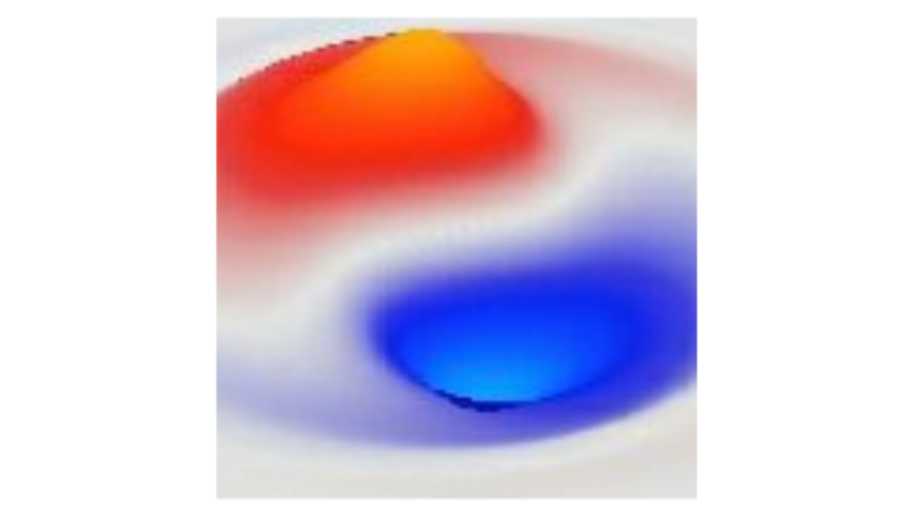
The Schrödinger wave equation captures non-relativistic Newtonian physics in a simple linear, first-order framework, and can be derived from a Hamiltonian representing the total energy of the system, which is strictly conserved over time. It captures the fundamental relationships between momentum and wave frequency at the heart of quantum physics, as discussed in Klein-Gordon.
As shown in complex waves (which is recommended to be read prior to continuing), the Schrödinger equation is the simplest omnidirectional first-order complex wave equation, and at its core, it is essentially just a rotation in the complex number plane. Indeed, the use of this equation in the Hilbert space framework is typically as a simple complex-plane rotation through the configuration space variables, using a more abstract, non-spatial definition of the time-invariant Hamiltonian, which reduces to specifying the energy that determines the rate of rotation:
\[ U(t) = e^{-iHt/\hbar} \]
(see rotation by the exponential for why this is a unitary rotation operator).
Compared to the full complexity of the gauge theory framework used in coupling the EM (Maxwell) field with a charged particle field like the Dirac equation, which is the basis for the Standard Model, this Schrödinger framework represents a significant simplification. Indeed, because the Schrödinger wave equation is linear, it is incapable of capturing particle interactions, because the waves simply superpose (additively combine) past each other, without impacting each other at all.
Thus, in order to capture relevant interactions, the Schrödinger wave equation requires the tensor-product, exponentially-large configuration space representation. For example, if there are two interacting particles in position space, then they each get their own set of 3D coordinates within this configuration space, and the entire wave function evolves over time so as to conserve the overall energy / probability represented in the configuration space. As such, configuration space is entirely non-local by construction, representing at each instant of time the entire configuration of the system, regardless of how far apart any of the particles might be.
Schrodinger’s equation
Using the total energy (Hamiltonian) approach, we can derive Schrödinger’s equation, using the same energy and momentum operators that we used in the derivation of the Klein-Gordon equation (strongly recommend reading that page first, for the introductory treatment of this approach). To remind, these operators are:
\[ \hat{p} = -i \hbar \vec{\nabla} \]
\[ \hat{E} = i \hbar \frac{\partial }{\partial t} \]
\[ \vec{\nabla} = \left(\frac{\partial {}}{\partial {x}}, \frac{\partial {}}{\partial {y}}, \frac{\partial}{\partial {z}}\right) \]
Next, we need to define the total energy Hamiltonian. Instead of the relativistic total energy, we use the classical Newtonian expression for the kinetic energy of a particle, in terms of its velocity \(\vec{v}\), just as we did in the simple wave energy calculation in waves:
\[ K = \frac{1}{2} m_0 \vec{v}^2 = \frac{1}{2 m_0} \vec{p}^2 \]
The second form uses the Newtonian relationship of momentum to velocity (just \(\vec{p} = m_0 \vec{v}\)) — because we have a momentum operator, we need to use this momentum form.
We also include a potential energy term that is a function of any kind of electrical or other force potential that the particle experiences. We won’t deal much with such forces at this point, so we just call this potential energy \(V\) for now, and focus on the kinetic energy. The total energy or Hamiltonian in abstract terms is just the kinetic energy \(K\) plus this potential energy:
\[ E = K + V \]
\[ E = \frac{1}{2 m_0} \vec{p}^2 + V \]
We can now just apply our momentum and energy operators to these expressions, and the result is in fact:
\[ i \hbar \frac{\partial \chi}{\partial t} = -\frac{\hbar^2}{2 m_0} \nabla^2 \chi + V \chi \]
The net result is that we can conclude that Schrödinger’s equation provides an accurate description of the flow of energy and momentum over time of a “particle” described by a wave, such that it obeys classical Newtonian physical laws. Note that in comparison with the KG equation, there is no speed-of-light factor \(c\) in this equation, consistent with its non-relativistic nature.
Omitting various constants (factors of \(\hbar\)) and any external force potential, Schrödinger’s equation is:
\[ i \frac{\partial \chi}{\partial t} = - \frac{1}{2m_0} \nabla^2 \chi \]
where \(m_0\) is again the rest mass of the particle in question. This is clearly very similar to the basic second-order KG wave equation:
\[ \frac{\partial^2 \phi}{\partial t^2} = c^2 \nabla^2 \phi - \frac{m_0^2}{\hbar^2} \phi \]
except that the temporal derivative is first-order, and mass enters in a different way. Nevertheless, the driving force is still the overall curvature of the wave, computed by \(\nabla^2 \phi\). As we noted above, the multiplication by the \(i\) term causes things to rotate — this rotation is key for making the first-order equation behave like a wave.
To see this effect more explicitly, we can write out Schrödinger’s equation in terms of the two underlying scalar values:
\[ i \frac{\partial ({\phi_a + i \phi_b})}{\partial t} = - \frac{1}{2m_0} \nabla^2 (\phi_a + i \phi_b) \]
\[ -\frac{\partial {\phi_b}}{\partial t} + \frac{\partial {i \phi_a}}{\partial t} = -\frac{1}{2m_0} \nabla^2 \phi_a - \frac{i}{2m_0} \nabla^2 \phi_b \]
where \(\phi_a\) indicates a scalar state variable that is the \(a\) component of \(\chi\), and \(\phi_b\) is the \(b\) component of \(\chi\). Note that the derivatives operate separately on each of the two variables. At this point, we now can just separate all the terms that involve an \(i\) from those that do not, to get update equations for each of the two variables. For the real-valued components (without the \(i\)):
\[ -\frac{\partial {\phi_b}}{\partial t} = - \frac{1}{2m_0} \nabla^2 \phi_a \]
\[ \frac{\partial {\phi_b}}{\partial t} = \frac{1}{2m_0} \nabla^2 \phi_a \]
and for the imaginary components (dropping the \(i\) now, because we no longer need it to keep the variables separated):
\[ \frac{\partial {\phi_a}}{\partial t} = - \frac{1}{2m_0} \nabla^2 \phi_b \]
In a discrete-space and time cellular automaton implementation, these equations would be written:
\[ \dot {\phi_a}_i^{t+1} = - \frac{3}{26 m_0} \sum_{j \in N_{26}} k_j ({\phi_b}_j^t - {\phi_b}_i^t) \]
\[ {\phi_a}_i^{t+1} = {\phi_a}_i^t + \dot {\phi_a}_i^{t+1} \]
and:
\[ \dot {\phi_b}_i^{t+1} = \frac{3}{26 m_0}\sum_{j \in N_{26}} k_j ({\phi_a}_j^t - {\phi_a}_i^t) \]
\[ {\phi_b}_i^{t+1} = {\phi_b}_i^t + \dot {\phi_b}_i^{t+1} \]
So, in the end, Schrödinger’s equation really just boils down to two very simple differential equations. Interestingly, these equations are coupled, in the sense that it is the curvature of \(\phi_a\) that drives the change in \(\phi_b\), and vice-versa. This is the rotational aspect of the equation mentioned earlier, which is caused by the presence of the \(i\) in the equation.
When you actually implement Schrödinger’s equation on a computer using the update rules given above, the resulting system is numerically unstable. In other words, the resulting numbers quickly blow up to infinity. This is not due to any kind of numerical roundoff error from limited precision floating point numbers on the computer, but rather due to the way that changes in state values reverberate back and forth across the two scalar values: it is a rotation being integrated by a method that does not rotate. The fix is to alternate the update: advance \(\phi_a\) using the old \(\phi_b\), then advance \(\phi_b\) using the new \(\phi_a\) (Visscher, 1991; Askar & Cakmak, 1978). This method is explicitly stable and second-order accurate, and is the only viable solution for a cellular automaton, because \(\phi_b\) depends on the neighboring cells’ \(\phi_a\).
The basic phenomenology of Schrödinger’s equation is that wave packets propagate through space, with a speed that is proportional to \(\nabla^2 \chi\), which in turn is proportional to the frequency of the wave. In other words, it describes exactly the same behavior as the KG equation, where particle speed is proportional to frequency.
One critical property of Schrödinger’s equation (which the scalar Klein-Gordon equation does not have) is that it preserves the overall magnitude of the \(\chi\) state values across all of space, for all time. This is to say, if you compute the sum of \(\chi \chi^*\) for each point in space, this sum will remain the same across time under the Schrödinger equation. This conserved value is interpreted as a probability in standard quantum mechanics. The alternating update conserves it too, but in a staggered form: because \(\phi_a\) and \(\phi_b\) are half a step apart in time, what is exactly constant is \(\phi_a^2 + \phi_b(t-1/2) \phi_b(t+1/2)\), rather than \(\phi_a^2 + \phi_b^2\).
For example, we can initialize the state with a localized wave packet (see matter waves) to represent the initial probability for the location and velocity of a particle (velocity being a function of the frequency of the wave packet). If we then apply the Schrödinger equation repeatedly, we can interpret the resulting \(\chi \chi^*\) values as the probability of the particle having moved to the corresponding location.
In other words, the wave packet defines a kind of “cloud of probability” for finding a discrete particle within its midst. However, these probabilities have different meanings in different scenarios, and it is notoriously difficult to come up with an intuitively sensible interpretation of what these probability clouds mean (see Copenhagen for discussion).
Explorations
See Schrodinger 1D Simulation and Schrodinger 3D Simulation for hands-on simulations.