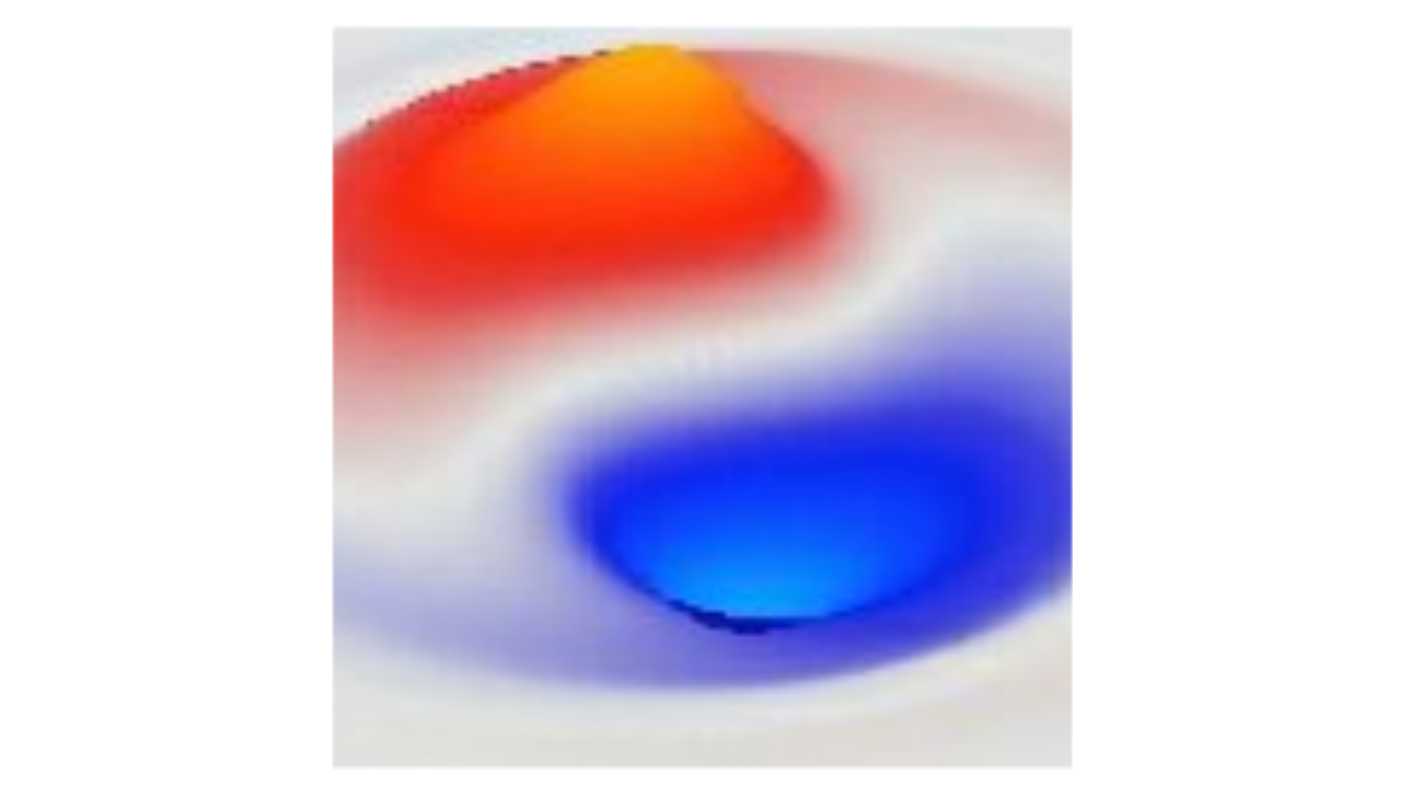
Gauge theory is the only mathematical framework that can tell us how a wave field that describes a particle (e.g., the Dirac field) should interact or couple with a force wave field, in a way that results in the conservation of overall energy and of the charge density (or probability density) of the particle field. Remarkably, there is really only one way to do this, and furthermore, this only way of doing it forbids writing down a mass for the force field, so it must be massless, like the simple second-order wave equation, and Maxwell’s equations for the electromagnetic field.
The reason is simple: the physical implications of the gauge field \(A_\mu\) are the same (i.e., invariant) if you add an arbitrary gradient. But if you would add such a gradient, the magnitude of the field (i.e., \(A_\mu A^\mu\)), is not invariant, and this is what a mass term would have to be based on. Thus, the value of the mass would change when nothing physical has changed. Because of this basic constraint, there is simply no legal way to write a mass into the theory by hand. The way that gauge theory gets around this is by having the mass arise through the interaction with the particle field, not as a direct factor in the force field itself.
This basic inability for a force field to have mass was among the most important challenges for physicists in the 1960’s, because both the weak and strong forces seemed to be massive, operating over a very short range, which is consistent with a massive field.
If these force fields are massive, then the mass term itself destroys the gauge invariance, and with it the conserved current!
One potential escape route was to somehow have mass emerge through a dynamic, emergent process, where it is technically not there in the equations, but it arises indirectly, for example via a spontaneous symmetry breaking process, where the lowest-energy solution that the system will naturally fall into ends up giving the force field a mass term. But that route appeared to be blocked too, by a result proven in the early 1960’s by Goldstone and collaborators (Goldstone, 1961; Goldstone et al., 1962):
Spontaneously breaking a continuous global symmetry necessarily produces a new massless scalar field.
These unwanted massless scalars are called Goldstone bosons, and in addition to being massless (and therefore necessarily associated with a long-range force), they are also scalar (spin 0), which means they cannot act like a force field.
So there were two walls. Gauge invariance forbids writing a mass in by hand, and spontaneous breaking of a global symmetry predicts a massless scalar field that does not exist.
The resolution is that when the symmetry is local (i.e., gauged) rather than global, the two problems cancel each other out: the would-be Goldstone scalar is absorbed into the force field, which thereby becomes massive, and no massless scalar is left over. This is the Higgs mechanism, and it leads to the full electroweak theory developed starting with Weinberg (1967).
For this all to work out, the Higgs field must have two complex-valued field components (i.e., 4 total numbers), which interact with no less than 4 different force fields. This is an example of a non-Abelian force field, which is a technical term from group theory in mathematics, but in physics this means that the force-field is self-interacting, as compared to an Abelian field like EM, which is not self interacting (i.e., the field is entirely linear and the only interactions are with the particle field, not amongst the field with itself).
Interestingly, the core mechanism behind this framework is actually already present in the most basic version of the Abelian gauge theory that we review below, and in some ways all the attention on the Higgs mechanism tends to distract from the essential nature of this solution. This solution was sketched in qualitative form already by Anderson (1963) and Schwinger (1962), based on inspiration from superconductors and other non-quantum systems (see Witten (2016) for an accessible history of these developments, and Poniatowski (2019) for a careful pedagogical treatment of the superconducting case).
The critical phenomenon is:
When the force and particle fields are coupled, there is a bidirectional self-interaction between these fields that ends up giving the force field an effective mass, in a way that depends on the magnitude of the particle field and the strength of the coupling!
This is an essential feature of gauge coupling, which is often overlooked in the QED (electron, EM fields) case, because the strength of this coupling between the two fields is relatively weak, on the scale of \(\alpha \approx 1/137\). So the EM field does not gain very much mass from this interaction, and it can generally be neglected. But if the coupling strength is significantly larger, then this fundamentally nonlinear effect can become much more significant.
Crucially, this effective mass does not violate gauge invariance, which is why it is allowed where a hand-written mass is not. The mass term that appears is proportional to \(|\chi|^2 A_\mu A^\mu\), but it never appears alone: it arrives packaged together with the phase of \(\chi\), and it is that phase which compensates for the non-invariance of \(A_\mu A^\mu\). This intimate coupling between particle and force fields is the necessary dance that makes it all work out, both for conservation principles and for the dynamic origin of mass. The resulting theory never stops being gauge invariant, and yet it develops a mass anyway. This was the key insight articulated clearly by Schwinger (1962).
This self-interaction mass effect is only present in the region where the particle field has a non-zero magnitude, because the effect derives from the charge current density of the field, which is a function of the field magnitude. This current density is what drives the force field (this is the source term of the standard Maxwell EM equations), and it represents one direction of the self-interaction. The other direction comes from an additional effect on the current arising from the field forces that this current itself generates. It is this additional effect that ends up generating the mass of the force fields in the electroweak framework.
The Higgs field plays the role of the particle source in the electroweak system, and it ends up providing the equivalent of a uniformly distributed charge current density throughout the universe. This uniformity is what makes the difference between a real mass and a mere local screening effect: an ordinary electron carries its little cloud of \(|\chi|^2\) around with it, so the effect dies away with distance and light far from the electron is unaffected, whereas the Higgs doublet has the same non-zero magnitude everywhere, so the effect never dies away and the force field acquires a genuine, permanent mass.
Furthermore, because the electroweak system is non-Abelian, there are no less than 4 different force fields (some of which mutually interact with each other), and the way the Higgs doublet’s own charges are assigned effectively creates one special configuration of these fields that actually remains massless, because the self-interaction terms end up canceling each other out, such that the current source density ends up being zero for such a configuration.
The result is that any waves that have this particular configuration will propagate over a long range, because they are effectively massless, while all the massive configurations will end up decaying over a relatively short range. Thus, the Higgs field acts much like a filter: the only thing that gets through is light itself (EM radiation over the effectively massless field configuration), while everything else is effectively the massive weak bosonic fields \(W^\pm\) and \(Z^0\).
In short, the inevitable mechanics of gauge coupling (the only possible way of doing things), which absolutely forbids a hand-written mass for the force fields, also happens to provide exactly the mechanism needed to generate an effective, dynamic type of mass, which also happens to allow exactly one effective force field to remain massless and long range, while the rest are massive and short-range. And all of this fits precisely with the empirical facts of the physical world we happen to live in. It is truly a mind-blowing situation, all stemming directly from the basic requirement of having force and particle fields interact in a conservative way. Hopefully that provides sufficient motivation to see how this all plays out!
Coupling between electron and electromagnetic fields
The principle of gauge invariance can be illustrated in the case of the electromagnetic force interaction with the electron represented in a simplified form by a complex wave state \(\chi\) obeying the complex KG wave equation (which is the simplest kind of wave state that can represent a conserved charge value). You should read the first part of that page, and then come back here where directed, when the EM coupling is addressed. You should also read the Lagrangian page, as that provides the mathematical framework upon which this is based (although we do cover enough to get by if you are impatient).
Throughout this section we use natural units (\(\hbar = c = 1\)) and a single generic coupling constant \(g\), in place of the specific electromagnetic \(e / \hbar c\) that appears in complex KG. This keeps the structure visible without the clutter, and it makes the result directly reusable for the weak coupling constants later on.
The analysis starts with a Lagrangian defined as the kinetic energy minus a potential energy for this electron field, where, in four-vector notation, the kinetic term is the product of the covariant and contravariant first derivatives of the wave function (contracted over all four space-time directions):
\[ \mathcal{L} = T - V \]
\[ \mathcal{L} = \partial_\mu\chi^*\partial^\mu\chi - V(\chi^* \chi) \]
Global gauge invariance
Notice that \(\chi\) only ever enters this Lagrangian paired with its own complex conjugate (i.e., as the magnitude). Therefore, multiplying the whole field by a constant phase \(G\) — a complex number of magnitude 1, the same everywhere — changes nothing at all, because the phase in \(\chi\) is exactly undone by the opposite phase in \(\chi^*\). If unfamiliar, see complex number for a review of how multiplication by \(e^{i\theta}\) can accomplish rotation in the complex plane, and rotation changes the phase of the field, which is the relative magnitudes of the two complex values.
\[ \chi \rightarrow \chi' = G \chi, \qquad G = e^{-i\theta} \]
where \(\theta\) is a constant. This global gauge transformation gives rise to a corresponding “symmetry” or invariance, which really means that something is unchanging or conserved. In this case, there is a conserved current (see continuity for the algebraic derivation), which critically involves multiplying the partial derivative of the field times the complex-conjugate of the field value, at every point:
\[ j^\mu = -i g \left[ \chi^*\partial^\mu\chi - (\partial^\mu\chi^*)\chi \right] \]
The constant in front is conventional, and the coupling factor \(g\) determines how strongly it would drive a force field.
The conserved nature of the current means that any accumulation of charge in a region is exactly accounted for by the current flowing across its boundary, so that the total charge integrated over all space never changes:
\[ \partial_\mu j^\mu = 0 \]
In more advanced versions (such as the electroweak case), you can introduce multi-component wave fields, and that allows the constant phase to be replaced by a matrix, \(G = e^{-i\theta^a T^a}\), where the generators \(T^a\) thereby determine the kind of symmetry group that the system obeys. This is basically where the Abelian vs. non-Abelian distinction arises: the generators either commute with each other or they don’t. For this case, with just a single-component complex field, there is a single generator and it corresponds to the simplest \(U(1)\) symmetry group.
Local gauge invariance
So far, we have only defined our electron, and shown that it can have a conserved current. But this current doesn’t do anything yet. This is just a free electron with no force field to interact with. The way that the force field is introduced in gauge theory seems very strange and somewhat arbitrary, and most treatments just plow right ahead without properly motivating the steps that come next. The whole point of this next step is to introduce the coupling with the force field in a way that still conserves the global current.
The way you do this is to first introduce a local factor (which ends up being the force field) that varies as a function of position and time, known as a local gauge transformation, and then observe that doing so really messes up your conserved current. This is because, unlike the case with the global transformation, this local transformation can change the slope of the wave field at any given point, and it therefore changes the partial derivative that enters into the current factor.
So what are you going to do to fix this mistake that you just made by introducing this force field? Well, you’re going to change the definition of the derivative in precisely the way necessary to undo the mistake, and restore your conserved current! This new form of the derivative defines a minimal coupling between the new force field and the particle field, and mathematically determines how to update the Lagrangian and the resulting laws of motion to specify this interaction between the two fields.
\[ \chi(x) \rightarrow \chi(x)' = G(x) \chi(x) \]
\[ G(x) = e^{-i \theta(x)} \]
where \(\theta(x)\) is now an arbitrary function specifying the phase of \(G(x)\) at every point – we will parameterize this with an additional field in a moment.
If you apply the covariant four-vector derivative to this transformed field, as required by the Lagrangian, you end up with an extra term from the product rule:
\[ \partial_\mu \chi \rightarrow G \partial_\mu \chi + \chi \, \partial_\mu G \]
This extra term means that the system is not invariant to this local gauge transformation, as we expected – no such system would be.
Now, you introduce a new gauge field that is going to represent the local transformation parameters, in the form of the electromagnetic vector potential field \(A_\mu(x)\), which shifts in the opposite direction, so as to absorb the extra term:
\[ A_\mu(x) \rightarrow A_\mu(x) - \frac{1}{g} \partial_\mu \theta(x) \]
where \(g\) is the coupling constant that parameterizes the strength of the interaction between this EM field and the original complex particle field.
Notice immediately what this shift costs us. The quantity \(A_\mu A^\mu\) is the only candidate for a mass term for the force field, and under this shift it becomes something else entirely. So a mass term for \(A_\mu\) is simply not available — this is the precise sense in which gauge invariance forbids a massive force field. Hold onto this, because we are about to find a mass anyway.
Next, we define our own new covariant derivative in a way that will make all the math work out under the local gauge transformation (dropping the explicit factors of x from now on):
\[ D_\mu \chi = \left(\partial_\mu - i g A_\mu\right)\chi \]
This works exactly as designed: the \(-\frac{1}{g}\partial_\mu\theta\) picked up by \(A_\mu\) generates a \(+i\partial_\mu\theta\,\chi\) that cancels the unwanted \(\chi\,\partial_\mu G\), leaving \(D_\mu\chi \rightarrow G\, D_\mu\chi\), which transforms exactly like \(\chi\) itself. Replacing \(\partial_\mu\) with \(D_\mu\) everywhere in the Lagrangian therefore restores the invariance, and with it the conserved current.
Finally, the force field needs its own kinetic term, so that it can propagate on its own rather than merely being carried along by \(\chi\). The unique gauge-invariant choice is built from the field strength \(F_{\mu\nu} = \partial_\mu A_\nu - \partial_\nu A_\mu\):
\[ \mathcal{L} = (D_\mu\chi)^*(D^\mu\chi) - V(\chi^*\chi) - \tfrac{1}{4}F_{\mu\nu}F^{\mu\nu} \]
Varying this with respect to \(A_\mu\) gives the wave equation for the potential, which (in the Lorenz gauge \(\partial^\mu A_\mu = 0\)) is driven by the current generated by \(\chi\):
\[ \square\, A_\mu = j_\mu \]
And the current itself is the same expression as before, with \(\partial_\mu\) replaced by \(D_\mu\):
\[ j_\mu = -i g \left[\chi^* D_\mu \chi - (D_\mu \chi)^* \chi\right] \]
Expanding the covariant derivative splits the current into two pieces:
\[ j_\mu = \underbrace{-i g\left[\chi^*\partial_\mu\chi - (\partial_\mu\chi^*)\chi\right]}_{\text{convection}} \;-\; \underbrace{2 g^2\,|\chi|^2 A_\mu}_{\text{proportional to } A} \]
The first term is conventionally described as a convection factor (or the paramagnetic current), and it corresponds to the original charge density that we started out with before introducing the covariant derivative. It depends on how \(\chi\)’s phase varies.
The second term is where the force field \(A_\mu\) is generating its own contribution to the current – the feedback factor for the force to the current. It is known as the diamagnetic or seagull term (because it looks like a seagull in certain representations; Minotti & Modanese, 2026; Figueiredo & Aguilar, 2016), and it has no counterpart in the free theory: it exists only because of the coupling. Critically, you can move this to the left hand side of the wave equation, and recognize that it operates just like the mass term in the KG equation!
\[ \square\, A_\mu + 2 g^2 |\chi|^2 A_\mu = j^{\text{conv}}_\mu \]
That is a Klein-Gordon equation for \(A_\mu\), driven by the convection current, with an effective mass given by:
\[ m_A^2 = 2 g^2 |\chi|^2, \qquad m_A = \sqrt{2}\, g\, |\chi| \]
We said above that \(A_\mu A^\mu\) cannot appear in the Lagrangian, because the gauge shift Eq 4 changes its value. Yet expanding \((D_\mu\chi)^*(D^\mu\chi)\) produces exactly \(g^2|\chi|^2 A_\mu A^\mu\). How is this possible?
The answer is that \((D_\mu\chi)^*(D^\mu\chi)\) is gauge invariant as a whole, but its individual pieces are not. The \(A_\mu A^\mu\) piece is not invariant by itself, and neither are the cross terms that couple \(A_\mu\) to the phase of \(\chi\). Their non-invariances cancel. So what looks like a mass term is really a mass plus a compensating scalar degree of freedom, namely \(\chi\)’s phase, and the two are inseparable. This intimate coupling between particle and force fields is really the secret to both conservation and mass, all in one!
The effective mass is the plasma frequency
Interestingly, this “dynamic mass” of the EM field is not some kind of crazy unknown exotic property. Instead, the mass expression in Eq 10 is known as the plasma frequency for a particle field that is filled with a relatively uniform density of charged currents, so that it behaves more like a fluid than discrete particles. Restoring conventional units, \(m_A\) becomes \(\omega_p / c\), where \(\omega_p\) is the familiar plasma frequency, and \(|\chi|^2\) becomes the charge carrier number density.
Light below this plasma frequency does not propagate at all, which is why radio waves reflect off the ionosphere and why metals are shiny.
A superconductor represents an intermediate case, where there is a uniform and persistent current, so the EM field acquires a real mass inside it. The relation \(j \propto -|\chi|^2 A\) derived above is the London equation of superconductivity, written down in 1935, decades before anyone spoke of a Higgs mechanism (London, 1935). The resulting mass \(m_A\) is the inverse London penetration depth, and its consequence is the Meissner effect: magnetic fields are expelled from the superconductor because a massive force field cannot propagate into it. This was one of the phenomena that inspired Anderson (1963) in thinking about how one might solve the central mystery of how to have a massive force field without imposing a mass directly.
The only thing the Higgs field adds to this picture is permanence and uniformity. A plasma or a superconductor gives the photon a mass in a particular region, at a particular temperature, because that is where the charge carriers happen to be. The Higgs doublet has a non-zero magnitude everywhere and always, so the mass it confers is a permanent property of the force fields rather than a property of a medium.
Symmetry groups
• SU(2) is the double cover of the 3D rotation group – spin! So SU(2) x U(1) is pretty much determined by any spinning thing interacting with a massless radiative field. Not a general principle as much as a necessary fact, given that fermions spin..
• SU(3) is another story..
• Proca is the 4-vector (vector boson) version of KG: it is what you get when you write a mass in by hand, and it is exactly the thing gauge invariance forbids.