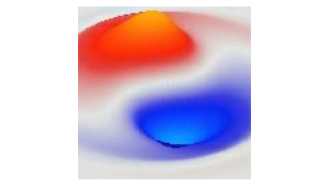
The Higgs field plays a central role in the weak interaction in the Standard Model, providing a mechanism for converting mathematically massless weak force bosons into the actual \(W^{\pm}\) and \(Z^0\) vector bosons that have (large) masses. Furthermore, the Higgs field also gives mass to the fermions through Yukawa coupling factors (Yukawa, 1935; wikipedia). Thus, the Higgs is unique in bidirectionally coupling with every other field, and filling the decidedly non-empty vacuum with four values per point that end up giving rise to the mass terms present in all the other fields. This mass term functions like the mass factor in the Klein-Gordon wave function, both for the Higgs field itself and for the other fields that it couples with, but instead of being a fixed parameter in an equation, it derives from the dynamics of the Higgs field itself.
At a metaphorical level, the Higgs field sounds sort of like a modern-day version of the aether, in its all-pervasive effects. These effects go well beyond just providing a single scalar mass value, due to the nature of the electroweak theory that integrates the weak force with the electromagnetic force, where the Higgs field plays a central (and very complex) role (Weinberg, 1967; Higgs, 1964; Englert & Brout, 1964; Guralnik et al., 1964).
The historical development of this whole framework originated because there is no way to accomplish the critical conservation trick performed by gauge theory using force-field bosons that have mass (Goldstone, 1961; Goldstone et al., 1962). That proved to be a major barrier in trying to understand the weak force, which was known to have a very short range of action, which strongly suggested that it is mediated by massive bosons. Surprisingly, it turns out that by doing all the math with massless bosons, and then adding the mass back in “at the end” in a very particular way, you end up with a sensible mathematical framework. And although this sounds suspiciously like a “hack”, it amazingly seems to accurately describe how the electroweak system actually works.
The key mechanism for being able to do the math with massless bosons, and then turning on the mass “at the end”, is through the spontaneous symmetry breaking in the Higgs field. The Higgs field is driven by the energy of all the other particles in a given region of space, and it also has a separate self coupling factor of a special form known as the Higgs potential. If the energy from all the other particles is sufficiently high, it effectively prevents the Higgs potential factor from having an effect, with the consequence that the average (expected) value of the Higgs field amplitudes is zero (as is the case for all the other fields, based on the basic nature of the wave equations).
However, once this background energy level goes below a critical threshold, the effective symmetry of the potential is broken, and the Higgs field takes on a vacuum expectation value determined by the Higgs potential, meaning that it now has a consistent effective mass. This threshold energy level is so high that the symmetry was effectively broken within the first 10 picoseconds after the big bang, so the symmetric case is effectively hypothetical for nearly the entire duration of the known universe. But, critically, this symmetric case is where the math all works, and, even though it really doesn’t look like it, the exact same math is operating in the post-symmetry breaking era as well.
Specifically, as shown in electroweak, the equations for the pre-symmetry-breaking version are relatively simple and elegant, but the post-symmetry-breaking case introduces significant complexity that only emerges once the Higgs field takes on a consistent expected mass value. It really is the same underlying math, but because the field couplings represent nonlinear interactions, extra terms emerge once the field stabilizes with a consistent mass. Mathematically, the same pre-symmetry-breaking equations are solved with a specific parameterization of this stable mass, which ends up being concentrated entirely in one of the four Higgs field values, as determined by the way these values interact in the electroweak system.
There are two related sources of inspiration for the Higgs mechanism, one from the Landau theory of phase transitions, for example based on the relationship between temperature and ferromagnetism, where at a sufficiently high temperature, the magnetic pole orientations in iron are bouncing around too much to stably align (Melo, 2017).
The other major inspiration comes from superconductivity (Goldstone, 1961; Goldstone et al., 1962; Nambu, 1960; Nambu & Jona-Lasinio, 1961; Dürr et al., 1959; Schwinger, 1962; Anderson, 1963). Superconductors can sustain electrical currents without any resistance (“friction”), and these electrical currents can then give rise to corresponding magnetic fields that cancel out any external magnetic fields inside the superconductor itself. Thus, phenomenologically, this illustrates how a long-range force (magnetism) can become short-ranged like the weak force, when it interacts with an “absorbing” medium. The Higgs field effectively plays this role as the absorbing medium, as a result of obtaining a non-zero mass value.
Higgs potential
The Higgs mechanism is based on the complex KG Klein-Gordon (KG) equation, where the complex values are necessary to have a conserved total magnitude of the state. Although the full version of the Higgs is deeply intertwined with the weak force, in the full electroweak system, we can describe a simple version of it here just to illustrate the basic idea of the Higgs symmetry breaking phenomenon.
In this simple case, we can even dispense with the complex state and just use a scalar wave state – in fact, the electroweak version ends up doing effectively the same thing in order to concentrate all of the mass into one component of the field, while keeping all the rest of the components at zero mass (but the complex version is needed for the gauge theory logic in coupling with the electromagnetic and weak boson fields).
First, we adopt a standard convention that the effective Higgs field values have a normalization factor applied to them, which is \(\frac{1}{\sqrt2}\) for the complex field values, and \(\frac{1}{\sqrt2}\) for the scalar \(\phi\) values that we’re using here.
Figure 1:
Higgs potential on a simple scalar value, and what that would look like in the complex plane, where there is a ring of equivalent mass magnitude at the minimum. The dashed-blue line shows what a positive \(\mu\) factor would look like, which is what happens when there is a very high temperature.
The general formula for the Higgs potential that shows up in the Lagrangian as a potential energy factor is written in this form:
\[ V(\Psi) = -\mu^2 \Psi^\dagger \Psi + \lambda (\Psi^\dagger \Psi)^2 \]
where the \(\Psi^\dagger \Psi\) expression represents the squared magnitude of the state value, by multiplying by the complex conjugate (see complex numbers; actually it is the Hermitian conjugate given the vector nature of the state – need to multiply by the transpose to just get the individual factors as essentially a dot product).
The \(\mu^2\) term is a mass-like parameter, like in the KG equation, except that it is negative (as asserted by the minus sign at the start). Anything with negative mass is like having a positive potential overall, which makes it unstable, by adding a consistent positive acceleration. The \(\lambda\) factor balances this out, but as a function of the squared magnitude. The full implications of this potential will become clearer as we proceed.
For our simple scalar example, we define:
\[ \Psi = \frac{1}{\sqrt2} \phi \]
Such that:
\[ V(\Psi) = -\frac{1}{2}\mu^2 \phi^2+ \frac{1}{4}\lambda (\phi^2)^2 \]
The form of this potential is a Mexican hat shape (cross section in the scalar case) (Figure 1), and we can solve for the minima / maxima of it by setting the first derivative of it to 0, to find the points where it is not changing:
\[ \frac{dV(\phi)}{d\phi} = -\mu^2 \phi + \lambda \phi^3 \]
This is 0 when \(\phi\) is 0, which ends up being a maximum in the resulting potential, and it also has another 0 point here:
\[ \phi^2 = \frac{\mu^2}{\lambda} \]
\[ \phi = \frac{\mu}{\sqrt{\lambda}} \]
This turns out to be the minimum point in the potential, and is where the wave equations will stabilize over time, if nothing else is going on to excite them. In other words, this value defines the vacuum expectation value of the Higgs field, which we denote as \(v_h\):
\[ v_h = \phi_{\min} = \frac{\mu}{\sqrt{\lambda}} \]
To incorporate this potential properly into the KG equation, we have to use the Lagrangian formulation, with the Euler-Lagrange equations that result in the equations of motion for the system. For a field-based system this results in the standard wave equation with an additional term based on the derivative of the potential:
\[ \partial^2 \phi = \nabla^2 \phi - \frac{dV(\phi)}{d\phi} \]
in effect, the Lagrangian is sensitive to how the potential changes as a function of changes in the wave state, which is intuitively why it shows up as a derivative. The resulting concrete wave equation is thus:
\[ \partial^2 \phi = (\nabla^2 + \mu^2 - \lambda \phi^2) \phi \]
As we already showed in Eq 2, these extra terms will be zero when \(\phi = v_h\), and the wave dynamics will naturally settle into that state over time as a stable equilibrium point, creating the non-zero vacuum expectation value that corresponds to a broken symmetry.
Table 1: Higgs parameter values
| parameter | value | \(\mu = m_h/\sqrt2\) | 88.47 GeV | \(\lambda = m_h^2/(2v^2)\) | 0.1291 | \(\phi_{\min} = \mu/\sqrt\lambda\) | 246.22 GeV \(= v\) | \(m_h = \sqrt2\,\mu = \sqrt{2\lambda}\,v\) | 125.11 GeV | \(V_{\min} = -\lambda v^4/4\) | \(-1.186\times10^8\) GeV⁴ | \(V = 0\) at \(\sqrt2\,v\) | 348.21 GeV |
|---|
The actual empirical values for these parameters are shown in Table 1 based on the current experimental data (Group, 2024).
The phase transition
Although everyone (e.g., Wikipedia sources) describes the Higgs mechanism in terms of spontaneous symmetry breaking as a function of the energy or temperature of the universe, the actual equations do not directly include anything that looks like a temperature or energy factor. This is because the actual impact of the kinetic energy (temperature) of particles enters via the coupling of fermions with the Higgs, in a way that is not evident directly in the basic equations as a temperature-like factor. So, when you stare at those equations, it looks like the symmetry is always going to be broken as long as there is any kind of activity present to knock the system off the peak of the Mexican hat.
However, temperature can be added directly into the potential equation by way of approximation based on what happens in the complete system (e.g., Weinberg, 1974), which in its simplest form looks like this:
\[ V(\Psi) = -(\mu^2 - T_c T^2) \Psi^\dagger \Psi + \lambda (\Psi^\dagger \Psi)^2 \]
Where \(T\) is the temperature and \(T_c\) is a coefficient based on the types of particles that are assumed to be around, which can be computed as:
\[ T_c = \frac{3 g^2 + g'^2 + 4 y_t^2 + 8 \lambda}{16} = 0.3973 \]
where these factors are explained in the weak equations, and are dominated by the heaviest particle which is the top quark, parameterized by its Yukawa coupling factor \(y_t\).
The simple algebraic point is that once \(T\) goes above a critical level, it cancels out the \(\mu^2\) factor, so that the overall mass-like factor is 0 or actually positive, and then the zero level of the field turns back into a minimum instead of an unstable maximum (as shown in Figure 1, in the dashed blue line). Thus, with this augmented form of the potential equation (which is purely for analysis purposes and doesn’t exist at the level of fundamental physics), it is hopefully clearer how the system can transition between the situation where the Higgs field has a 0 expected value (high temperature) versus one where it has a non-zero (massive) expected value (temperature below the critical level).
The critical value of the temperature is when it crosses the \(\mu^2\) value:
\[ T_{\text{critical}} = \frac{\mu}{\sqrt{T_c}} \]
Exploration
See the electroweak simulation for a hands-on exploration of the Higgs potential, in the context of the full electroweak system.
Fine tuning / hierarchy problem
Because the Higgs field couples with all particles according to the Standard Model, the strength of the Higgs field, i.e., the mass of the Higgs boson, should be a function of the masses of all of the different types of massive particles. Now that the mass of the Higgs boson has been measured, it can be used in reverse to compute the expected masses of all particles, including any that have yet to be discovered! The contribution of any given particle to the Higgs mass is (see Wikipedia):
\[ \Delta m^2_H = - \frac{|\lambda_f|^2}{8 \pi^2} [\Lambda_{\text{UV}}^2 + \dots] \]
Where \(\lambda_f\) is the Yukawa coupling factor, and \(\Lambda_{\text{UV}}^2\) is the ultraviolet cutoff energy. Thus, we can use the actual Higgs mass to determine the associated ultraviolet cutoff energy (Bezrukov & Shaposhnikov, 2015). The value of \(\lambda_f\) can be computed from the Higgs field energy:
\[ \lambda_f = \sqrt{2} m_f / v_h \]
where \(v_h\) is the vacuum expectation of the Higgs field, per above (246.22 GeV).
The heaviest currently-known fermion is the top quark, which weighs in at around 172 GeV, which means that its \(\lambda_f\) is 1, which is consistent with existing measurements (Collaboration, 2026). Thus, using Eq 4, we can compute that the ultraviolet cutoff implied by this mass is less than \(2 \sqrt{2} \pi\) times the Higgs boson mass, which is 8.89 times 125 GeV = 1,111 GeV. This suggests that the UV cutoff length scale is roughly in the \(10^{-18}m\) range, applying this GeV energy to the Planck relation.
This length scale is in the range of the weak force, which operates around the \(10^{-18}m\), and is well above the Planck length scale of \(10^{-35}m\), where gravitation is as strong as EM. Thus, consistent with the application of the renormalization procedure, the Higgs mass is consistent with the Standard Model being a complete model, with no room for additional higher-energy (mass) particles, etc.