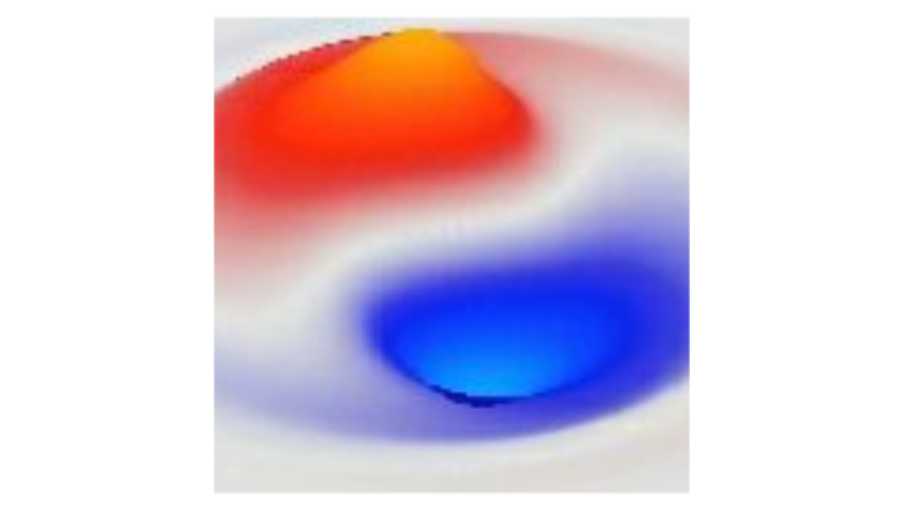
The second-order wave equation is the prototypical version of a wave, which corresponds to macroscopic water waves and other such familiar phenomena. The core dynamic in such waves is the continuous bidirectional conversion of energy between wrinkles in space (potential energy) and movement through time (kinetic energy). However, standard quantum mechanics is based on Schrodinger waves, which obey a first-order equation that uses the rotational properties of complex numbers instead of the second-order integration of kinetic-energy to accomplish the core oscillatory property of waves.
The ability to capture oscillations through either a second-order kinetic system, or a first-order complex-number system, plays out in various ways throughout the larger space of quantum wave equations. Here, we develop a systematic understanding of this space, and the relative tradeoffs between these different wave functions.
Of primary interest is the extent to which the different wave equations tend to spread out over time (known as dispersion, which is also related to diffraction), because that relates to the epistemic vs ontological aspect of what the wave is describing: as a wave propagates, the uncertainty in where it is going should generally increase, especially to the extent it exhibits stochastic motion. This is purely epistemic: our knowledge of it becomes less precise, but, under the pilot wave framework, a discrete particle should be localized precisely at all times, and its surrounding quantum wave should presumably not spread out.
Figure 1:
Dispersion for three different wave equations with identical parameters, showing qualitative differences consistent with the analysis here. WidMagX records the width of the wave packet in the longitudinal direction that the wave is moving, while WidMagZ is the transverse width in the Z axis. For all cases, the transverse dispersion (also known as diffraction) is greater than the longitudinal. Because the Schrödinger equation is essentially a diffusion equation driving complex rotation, it has the highest rate of dispersion by far. The second-order Dirac equation (which performs the same as the basic Klein-Gordon wave equation) avoids the diffusion dynamic of the Schrödinger. The first-order, complex Weyl equation minimizes dispersion by driving complex rotation in a fixed rotational direction.
Thus, if we can find wave equations that differ in their tendency to spread out (as shown in Figure 1), this may have implications for the kinds of waves we might want to be using for a pilot-wave model. One interesting conclusion from this analysis is that the neutrino could be seen as a kind of necessary byproduct of a type of first-order electron waves that don’t spread out as much as they do in the second-order wave function (described by the Weyl equation, which is what is necessary for the electroweak framework). Furthermore, the Schrödinger wave function lies at the other extreme end of the spectrum in terms of its tendency to spread out, which would seem to have major implications for all of the abstract quantum math based on it.
Before proceeding, it is particularly useful to first read the harmonic oscillator page, which provides a simple and direct comparison between a second-order kinetic version of an oscillator, and a first-order complex-number version of the same oscillator dynamics. This harmonic oscillator has a single spatial value (i.e., within a single isolated cellular automaton cell), so its spatial dimensionality is much simpler than the wave, especially when it spreads over 3D space. That makes it easier to see the fundamental difference in the way the time dimension works, which is the key difference between the first and second-order wave equations.
The natural starting point with respect to dispersion is with a second-order wave equation configured instead to implement the diffusion equation. This is a very simple change in the equation, which also reveals the essential role of the second-order acceleration in driving the oscillatory behavior of the wave equation. The change is to couple the spatial curvature (potential energy) directly to the velocity (first order), without going through the acceleration (second order).
\[ \frac{\partial^2 \phi}{\partial t^2} = c^2 \frac{\partial^2 \phi}{\partial x^2} \]
\[ \frac{\partial \phi}{\partial t} = c^2 \frac{\partial^2 \phi}{\partial x^2} \]
When you run this equation (you can do it in the wave simulation) you see any disturbance melt away over time – any “concentration” of wave “stuff” simply diffuses down into a uniform splat.
This is an interesting starting point, because the first-order Schrödinger equation is effectively the same as the diffusion equation, except it operates on complex state variables, and it sticks an \(i\) in there to drive the rotation.
\[ \frac{\partial \chi}{\partial t} = i \frac{\partial^2 \chi}{\partial x^2} \]
where \(\chi = \phi_a + i \phi_b\) is a complex-valued wave state with the two underlying values, which are just ordinary numbers. Although everyone somehow gets hung up on the \(\phi_b\) number being “imaginary”, it is just a regular number that happens to be located on an orthogonal plane to the “real” number, so that these two numbers can rotate around each other in qualitatively the same way that velocity and the state position value do in the second-order version of the wave equation.
Is the velocity in a second-order equation “imaginary”? No. It is just another degree of freedom – a different value that you can use to make things oscillate. The connection between rotation and oscillation is basic trigonometry: the sine and cosine are waves that arise in any orthogonal basis coordinates as you rotate around a circle, and the complex plane just provides a 2D space for this rotation to occur.
To understand exactly what is happening in Eq 3, we can write it in terms of the two ordinary numbers. The key algebraic step is that you only keep the factors without an \(i\) for the \(\phi_a\) factor, and those with an \(i\) for the \(\phi_b\) factor. Furthermore, the convenient fact that \(i^2 = -1\) makes the signs work out correctly for the rotation. The net result is that the \(i\) factor makes \(\phi_a\) depend on \(\phi_b\) and vice-versa – it causes the two values to rotate into each other:
\[ \frac{\partial \phi_a}{\partial t} = - \frac{\partial^2 \phi_b}{\partial x^2} \]
\[ \frac{\partial \phi_b}{\partial t} = \frac{\partial^2 \phi_a}{\partial x^2} \]
From the perspective of the second-order wave equation (Eq 1), the Schrödinger equation is a bit strange, because the spatial factor on the right-hand side is a second-order spatial derivative (also written as \(\nabla^2 \phi\) where \(\nabla^2\) is the Laplacian).
The critical advantage of this second-order spatial derivative is that it doesn’t care about direction: a spatial disturbance in any direction surrounding a given point in the wave state will give rise to a change in that wave state, proportional to the magnitude of the disturbance. This means that this equation supports waves traveling in any direction, just like the standard second-order wave equation, because that directional property depends entirely on the nature of the spatial derivative factor.
However, the coupling of this second-order spatial factor directly to the first-order temporal derivative in the Schrödinger equation results in an extremely high level of dispersion as shown in Figure 1. By contrast, the Klein-Gordon and Dirac equations, because they are second-order, avoid a significant amount of this dispersion, but nevertheless still inevitably exhibit some dispersion because of the omnidirectional nature of the Laplacian.
By following this logic to its logical conclusion, we should be able to significantly reduce the dispersion by using a first-order gradient instead of the omnidirectional Laplacian. But this would mean that the wave can only go in one direction, depending on which direction the gradient is being computed in:
\[ \frac{\partial \phi_a}{\partial t} = 2 c \frac{\partial \phi_a}{\partial x} \]
\[ \frac{\partial \phi_b}{\partial t} = 2 c \frac{\partial \phi_b}{\partial x} \]
Note that these two complex components are updated completely independently, so the wave state must be initialized with them 90 degrees out of phase. The spatial gradient on the right must be computed with respect to a specific basis vector, which is fixed to the X axis in the way it is implemented in the wave 3D simulation. Thus, this equation only describes waves that move either to the right or the left along one vector direction.
Clearly, this fixed directionality is a significant limitation, but it provides a useful bridge to the Weyl equation, which is able to preserve this gradient-driven dynamic, but by using a helical pattern of rotation, it can move in any direction! Specifically, there are two different Weyl equations, one for right-handed helicity and another for left-handed. The right-handed version involves a systematic pattern of rotation through the set of four real values in the Weyl wave state (two complex numbers), while the left-handed version rotates the other way.
When coupled via the Pauli matrices (the same ones that drive spin in the Dirac equation under the influence of the magnetic field), all three spatial directions of the first-order partial derivative enter into each update equation. For example, here is the update equation for the 1a component of the right-handed case:
\[ \frac{\partial \phi_{1a}}{\partial t} = - c \left( \frac{\partial \phi_{1a}}{\partial z} + \frac{\partial \phi_{2a}}{\partial x} + \frac{\partial \phi_{2b}}{\partial y} \right) \]
Thus, because each spatial gradient is present, the wave can then propagate along any weighted combination of these three spatial axes, meaning that the wave can move in any arbitrary direction. However, the pattern of rotation among the complex-valued elements has a characteristic ordering relative to the direction of wave travel, which is what defines the helicity of the equation.
Furthermore, each separate helicity in the Weyl system naturally propagates at the speed-of-light. This corresponds to the behavior of the neutrino (if considered to be massless, which it is actually not). However, if a mass term is present, it serves to couple the two separate helicities together, such that they now also rotate back and forth between each other, which has the net effect of slowing down the overall movement in each.
Thus, the Weyl system also provides a novel way for mass to enter into the wave equation, distinct from that present in the Schrodinger or Klein-Gordon frameworks. And the fact that it naturally gives rise to a massless case with a fixed helicity essentially predicts the existence of the neutrino!
There is, however, the important caveat that, in fact, neutrinos do have mass, which remains to be resolved with the rest of the Standard Model and the electroweak framework.
Figure 1 shows that the Weyl equation for an electron, coupling the left and right helicities with the electron mass, exhibits the lowest levels of dispersion, consistent with the use of the directional first-order gradient instead of the omnidirectional Laplacian.
In summary, you hopefully now have a deeper understanding of the dynamics and tradeoffs between these different forms of wave equations. Their different dispersion properties certainly raise questions about the use of the highly-dispersive Schrödinger equation in comparison to the Weyl equation.