
Complex KG
In Klein-Gordon we saw that a major problem with the scalar KG equation is that it doesn’t represent any kind of conserved value: you cannot compute some constant, unchanging value from the \(\phi\) state variables under this equation. This is a problem if you want to develop a probabilistic interpretation of the wave, as in Schrodinger’s equation for the standard Copenhagen interpretation. But it is also a problem for other interpretations as well. See conservation for an essential overview.
In particular, we would like the KG waves to represent waves of charge (i.e., matter waves), because charge is also strictly conserved, and it comes in both positive and negative varieties, which the KG waves produce. By contrast, the Schrödinger wave only represents a positive-valued quantity, which fits better with the probabilistic interpretation. Indeed, the authors that do write extensively about the KG equation adopt this interpretation (Greiner, 2000; Gingrich, 2004; Mandl & Shaw, 2013), and this idea was pursued initially by Schrödinger in 1926. Furthermore, we will see that this charge interpretation fits naturally with the coupling of this KG equation to the electromagnetic (EM) field (Maxwell’s equations), where the conserved charge value acts just like the electric charge in driving the field.
The critical step for transforming the KG equation into something that can represent a conserved charge value is to simply have it operate on wave state with complex numbers instead of scalars! The reason is at once simple and yet deeply profound for the nature of the quantum realm:
Complex numbers naturally maintain a constant radius as they rotate around the complex plane.
It is this constant radius value that corresponds to the conserved charge value in the complex KG wave equations. This radius is the hypotenuse of the triangle formed by the real and imaginary components of the complex number. According to the Pythagorean theorem, it is computed by the sum of the squared values. In the language of complex numbers, this is computed by multiplying by the complex conjugate, and we’ll see that this is how we compute the conserved charge value.
Once we have the ability to compute charge from the complex KG wave equations, then we can drive the electromagnetic field using that charge as a source. In order to do this, we need to apply the gauge theory technique of local gauge invariance, which is known as scalar electrodynamics in the case of coupling with a spinless complex charge field, as we are doing here (the term scalar can be used to distinguish from spin, or complex values, depending on the context). To make this work, we actually need 2 complex-valued state variables, to align with the four values of the electromagnetic four-potential \(A^\mu\).
Interestingly, this is actually a good model of how the Higgs mechanism works, because it involves precisely such a coupling between a spinless complex field and the gauge vector boson field \(B^\mu\) that works just like the electromagnetic four-potential \(A^\mu\).
However, to model the behavior of fermion particles, the wave function needs spin, which is what the Dirac wave function adds on top of the KG waves. This coupling of charge waves and EM waves has been pursued more recently in neoclassical self-coupled field theory (Jaynes & Cummings, 1963; Crisp & Jaynes, 1969; Barut & Van Huele, 1985; Barut & Dowling, 1990; Crisp, 1996; Finster et al., 1999; Radford, 2003; Masiello et al., 2005). It is pedagogically useful to incrementally develop this scalar (non-spinning) version of electrodynamic interactions first, and then introduce the further complexities of spin in the Dirac equation.
Complex state and conserved charge
The first step is to introduce a wave state with complex numbers (\(\chi\)) instead of scalars (\(\phi\)), which then supports the computation of a conserved quantity across the two complex state values. When we translate this complex wave function into two separate second-order wave equations without an \(i\) imaginary number factor, the KG equation is identical to computing two separate KG equations on each of the two scalar values represented by the complex state variable (i.e., \(\phi_a\) and \(\phi_b\)). This is different from Schrödinger’s wave equation, which is first order and has an \(i\) term that causes the \(a\) and \(b\) terms to intermix as the wave unfolds. See complex waves for more discussion of these differences.
\[ \frac{\partial^2 \chi}{\partial t^2} = (\nabla^2 - m_0^2) \chi \]
Because differentiation operates independently on the two separate scalar variables in a complex number, this is equivalent to two parallel scalar KG equations, which we can write as:
\[ \frac{\partial^2 \phi_a}{\partial t^2} = \left( \nabla^2 - m_0^2 \right) \phi_a \]
\[ \frac{\partial^2 \phi_b}{\partial t^2} = \left( \nabla^2 - m_0^2 \right) \phi_b \]
where again the \(\phi_a\) indicates a scalar state variable representing the real \(a\) component of \(\chi\), and \(\phi_b\) represents the imaginary \(b\) value.
Ok, so how do you get a charge out of that, so to speak? As with Schrödinger’s equation, the procedure involves multiplying by the complex conjugate (\(\chi^* = \phi_a - i \phi_b\)), which generally produces the overall magnitude or length of the vector represented by the two components of the complex number: \(\phi_a^2 + \phi_b^2\). If you compute the sum of the “squared” (complex conjugate multiplied) wave values across all of space (actually an integral, using continuous equations), and set its time derivative equal to zero (so that it never changes), you end up with an expression for the density and motion (current) of a quantity that is conserved (i.e., the charge).
The details of this process are shown in the derivation of the continuity equation. The resulting expression for computing the density of charge (typically written as \(\rho\), which is the Greek letter “rho”), which is to say, the amount of charge per cubic state unit, is:
\[ \rho \equiv \frac{i \hbar e}{2m_0c^2} \left( \chi^* \frac{\partial \chi}{\partial t} - \chi \frac{\partial \chi^*}{\partial t} \right) \]
where the \(e\) value is a constant (1.6e-19 in SI units) that converts natural units into proper units of charge.
This can be expressed in terms of the underlying scalar state variables that make up the complex state (\(\chi = \phi_a + i \phi_b\)), and their first temporal derivatives (\(\dot \phi_a\) and \(\dot \phi_b\)), and using natural units where \(c=\hbar=1\), as:
\[ \rho_i = \frac{e}{m_0} ({\phi_b}_i \dot {\phi_a}_i - {\phi_a}_i \dot {\phi_b}_i) \]
This is directly computable for each cubic cell \(i\) in the system.
It becomes clear when explicitly written out in this manner that charge represents a coupling of the two otherwise independently-updated variables in the complex number, and this suggests why a single scalar number cannot represent a conserved charge value.
Complex charge
totalTime := 100
ai := 1.0
bphase := 90.0
c := 1.0
mass := 0.1
hbar := 0.5
e := 1.0
csq := c * c
mcOverHSq := (mass * mass * csq) / (hbar * hbar)
heOverMCSq := (hbar * e) / (mass * csq)

var bphaseStr, massStr, hbarStr, msgStr string

##
sa := zeros(totalTime)
sb := zeros(totalTime)
da := zeros(totalTime)
db := zeros(totalTime)
chg := zeros(totalTime)
##

func valUpdate() {
    csq = c * c
    mcOverHSq = (mass * mass * csq) / (hbar * hbar)
    heOverMCSq = (hbar * e) / (mass * csq)
    bphaseStr = fmt.Sprintf("b phase: %4.0f", bphase)
    massStr = fmt.Sprintf("mass: %4.1f", mass)
    hbarStr = fmt.Sprintf("hbar: %4.1f", hbar)
    bi := ai * float64(math32.Cos(math32.DegToRad(float32(-bphase))))
    bvi := c * math.Sqrt(mcOverHSq) * ai * float64(math32.Sin(math32.DegToRad(float32(-bphase))))

    ##
    ap := array(ai)
    bp := array(bi)
    av := array(0.0)
    bv := array(bvi)
    for t := range totalTime {
        sa[t] = ap
        sb[t] = bp
        da[t] = av
        db[t] = bv
        chg[t] = heOverMCSq * (bp * av - ap * bv)

        av -= csq * mcOverHSq * ap
        ap += av

        bv -= csq * mcOverHSq * bp
        bp += bv
    }
    ##
    msgStr = fmt.Sprintf("<b>Charge: %7.3g </b>", chg.Float(99))
}

valUpdate()

plotStyler := func(s *plot.Style) {
    s.Plot.XAxis.Label = "Time"
    s.Plot.XAxis.Range.SetMax(100).SetMin(0)
}
plot.SetStyler(sa, plotStyler)

fig1, pw := lab.NewPlotWidget(b)
al := plots.NewLine(fig1, sa)
dal := plots.NewLine(fig1, da)
bl := plots.NewLine(fig1, sb)
dbl := plots.NewLine(fig1, db)
chgl := plots.NewLine(fig1, chg)
fig1.Legend.Add("a", al)
fig1.Legend.Add("av", dal)
fig1.Legend.Add("b", bl)
fig1.Legend.Add("bv", dbl)
fig1.Legend.Add("chg", chgl)

msgTx := core.NewText(b)
msgTx.Styler(func(s *styles.Style) {
    s.Min.X.Ch(80) // clean rendering with variable width content
})
core.Bind(&msgStr, msgTx)

func updt() {
    valUpdate()
    al.SetData(sa)
    dal.SetData(da)
    bl.SetData(sb)
    dbl.SetData(db)
    chgl.SetData(chg)
    msgTx.UpdateRender()
    pw.NeedsRender()
}

func addSlider(label *string, val *float64, mnVal, mxVal float32) {
    tx := core.NewText(b)
    tx.Styler(func(s *styles.Style) {
        s.Min.X.Ch(40)  // clean rendering with variable width content
    })
    core.Bind(label, tx)
	sld := core.NewSlider(b).SetMin(mnVal).SetMax(mxVal).SetEnforceStep(true)
    if mxVal > 10 {
        sld.SetStep(10)
    } else {
        sld.SetStep(0.1)
    }
	sld.SendChangeOnInput()
	sld.OnChange(func(e events.Event) {
		updt()
		tx.UpdateRender()
	})
	core.Bind(val, sld)
}

addSlider(&bphaseStr, &bphase, -180, 180)
addSlider(&massStr, &mass, 0.1, 1.0)
addSlider(&hbarStr, &hbar, 0.1, 1.0)
Sim 1 demonstrates how this works, in terms of two simple harmonic oscillator variables a and b, which are set to be a specific phase apart from each other (+90 degrees shifts b to the left (earlier) relative to a, while -90 shifts to the right, due to the trigonometric convention of 0 degrees being at 1,0 and proceeding counter-clockwise from there). Regardless of the phase relationship, the computed charge value remains constant across the cycles of oscillation. However, critically, the value of the charge is directly a function of this phase relationship, with a maximum of 1 (in units of e, for a unit amplitude wave) when the b value is +90 degrees in relation to the a value, and a minimum of -1 for -90 degrees, and zero for 0 or 180 degrees. These relationships are fairly obvious once you appreciate the relationship between velocity and position for each of the variables (which are 90 degrees out of phase with each other, always), and how they enter into the charge equation.
Critically, complex numbers are always 90 degrees out of phase with each other by the very nature of the complex plane. Thus, even though the separate real-valued wave functions are independently updated, it is critical that these two wave states are initialized with the 90 degree phase relationship appropriate for complex numbers, which will then determine the sign of the charge value represented.
Perhaps the most important feature of this charge equation is that it can be either positive or negative, as a function of the phase relationship. This is not true of the corresponding expression for Schrödinger’s equation, which is “definitely positive”, or, in mathematical terminology, “positive definite”. This is one of the major reasons why standard quantum physics has strongly embraced Schrödinger’s equation, and not KG: KG does not fit with the standard probabilistic framework, where the wave describes a probability, and a probability is always positive.
Interestingly, the Dirac equation, which is used in the Standard Model for all fermion particles such as the electron, also produces negative “probabilities”, but these have been (correctly, in our framework) reinterpreted as representing antiparticles (i.e., particles with an opposite charge). The antiparticle of the electron is the positron, and it is just like an electron, except it has the opposite charge. Historically, this antiparticle nature of the Dirac equation was regarded as a major problem, until positrons were subsequently discovered, and then Dirac looked like a genius for having made such a bold prediction.
We can also derive an expression for the motion of charge over space, which is the charge current density \(\vec{J}\):
\[ \vec{J} \equiv - \frac{i \hbar e}{2m_0} \left( \chi^* \vec{\nabla} \chi - \chi \vec{\nabla} \chi^* \right) \]
In terms of the underlying scalar state variables (and again for natural units), this is:
\[ \vec{J} = \frac{e}{m_0} (\phi_a \vec{\nabla} \phi_b - \phi_b \vec{\nabla} \phi_a) \]
This value indicates how much charge is moving in each of the three different coordinate directions; the \(\vec{}\) symbol on top of \(\vec{J}\) indicates that this is a vector, containing a separate real scalar value for each direction: \(\vec{J} = (J_x, J_y, J_z)\). The \(\vec{\nabla}\) symbol is the vector gradient operator, which computes the rate of change of the values along each dimension:
\[ \vec{\nabla} \equiv \left(\frac{\partial}{\partial x}, \frac{\partial}{\partial y}, \frac{\partial }{\partial z}\right) \]
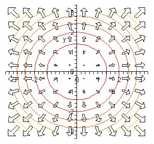
Figure 1: The gradient of a scalar field (\(\vec{\nabla}\)), which produces a vector field describing the slope at each point in space. These gradient vectors point in the direction of maximum ”downhill” slope. In this example the scalar field is a circularly-symmetric bump.
This just means that this \(\vec{\nabla}\) takes a three-dimensional field, in this case the field of our wave value \(\phi_a\) or \(\phi_b\) distributed over space, and computes how steeply this field is changing in each of the three different directions (Figure 1). See discrete gradient for how we compute the gradient \(\vec{\nabla}\) in discrete space-time of the cellular automaton framework.
Before proceeding, we look ahead to the next major development. We have ways of computing the density and current of charge (\(\rho\), \(\vec{J}\)), which drive the electromagnetic field. Thus, we can think of these as physically real values, which can be computed directly from the underlying wave state variables, that give rise to long-range electromagnetic forces, through which the particle-waves interact. The next step is to see how the electromagnetic fields can push our particle waves around.
To summarize, the computation of the current, which is a vector having three separate components (\(J_x, J_y, J_z\)), looks like this:
\[ J_x = \frac{e}{m_0} \left[ \phi_a \left( \sum_{j \in N_{X}} k_j ({\phi_b}_{j+} - {\phi_b}_{j-}) \right) - \phi_b \left( \sum_{j \in N_{X}} k_j ({\phi_a}_{j+} - {\phi_a}_{j-}) \right) \right] \]
\[ J_y = \frac{e}{m_0} \left[ \phi_a \left( \sum_{j \in N_{Y}} k_j ({\phi_b}_{j+} - {\phi_b}_{j-}) \right) - \phi_b \left( \sum_{j \in N_{Y}} k_j ({\phi_a}_{j+} - {\phi_a}_{j-}) \right) \right] \]
\[ J_z = \frac{e}{m_0} \left[ \phi_a \left( \sum_{j \in N_{Z}} k_j ({\phi_b}_{j+} - {\phi_b}_{j-}) \right) - \phi_b \left( \sum_{j \in N_{Z}} k_j ({\phi_a}_{j+} - {\phi_a}_{j-}) \right) \right] \]
Again, it does not look as simple as before, but nevertheless it is necessary to have a current to be able to drive the magnetic field in a manner consistent with known physics. Specifically, the electromagnetic field equations require both \(\rho\) and \(\vec{J}\) values as their sources (see Maxwell). In addition, this gradient operation is necessary for several other computations in our model, so, like the laplacian, it can be thought of as one of just a few basic operations that take place over the neighborhood of cells.
Minimal Coupling of Charge Waves with Electromagnetic Fields
At this point, we have a charged wave that can generate an electromagnetic field according to the charge density \(\rho\) and current density \(\vec{J}\), and we know how this electromagnetic field propagates according to the Maxwell wave equations. Now, we need to have that electromagnetic field interact with the charge wave to produce actual forces on a charged particle. This occurs by introducing new terms into the complex KG wave equation, which, intuitively speaking, act as external driving forces on this charge wave, in much the same way that the charge and current act as driving forces on the electromagnetic wave equations.
In the electromagnetic field equations, the driving force from charge \(\rho\) adds into the second-order temporal derivative \(\frac{\partial^2}{\partial t^2}\) (Eq 3 in Maxwell):
\[ \frac{\partial^2 {A_0}}{\partial t^2} = \nabla^2 A_0 + \frac{1}{\epsilon_0} \rho \]
However, in Schrödinger’s equation, external forces enter as a potential (\(V\)), in the first-order derivative \(\frac{\partial}{\partial t}\):
\[ i \hbar \frac{\partial {\chi}}{\partial t} = -\frac{\hbar^2}{2m} \nabla^2 \chi + V \chi \]
This makes sense, because force is the derivative of a potential, so potential is a first-order factor, and force is a second-order factor.
Our KG (Klein-Gordon) charge wave equation is a second-order equation, expressed in terms of \(\frac{\partial^2}{\partial t^2}\), and therefore we need to include external driving forces, not potentials. However, for various reasons, it is necessary to derive such an equation starting from the potential. To do this, we can re-derive a second-order wave equation by replacing the first-order derivative with the following first-order covariant derivative operator \(D\), that incorporates the external driving potential:
\[ D_\mu \equiv \partial_\mu + i \frac{e}{\hbar c} A_\mu \]
This derivative can be derived from the principle of local gauge invariance, in gauge theory, as a way to compensate for the introduction of a local phase factor, which is parameterized by the \(A^\mu\) potential field. In other words, local gauge invariance means that the EM field potential might be different at every different point in space, and gauge theory shows you how to have the EM field and charge field interact in a way that makes this situation mutually compatible, so that charge and energy end up being conserved over time.
We can then substitute this first-order four-vector derivative, and its contravariant version with the negative space-like factors, into the four-vector version of the KG wave equation (in natural units), which is (Eq 4 in Klein-Gordon):
\[ \partial_\mu \partial^\mu \chi = - m_0^2 \chi \]
because, as we’ve noted before:
\[ \partial_\mu \partial^\mu = \frac{\partial^2}{\partial t^2} - \nabla^2 \]
So the compact form of the KG wave equation with minimal coupling (local gauge invariance) is therefore:
\[ \left( \partial_\mu + i e A_\mu \right) \left(\partial^\mu + i e A^\mu \right) \chi = -m_0^2 \chi \]
To get all the units right, and perhaps add some conceptual clarity, we can do the same thing with the four-momentum version of the wave equation, which is:
\[ \hat{p}^\mu \hat{p}_\mu \chi = m_0^2 c^2 \chi \]
where the momentum operator is essentially just the four-derivative, plus the pesky \(i\) and \(\hbar\) factors:
\[ \hat{p}^\mu = i \hbar \partial^\mu \]
So now we can say that the electromagnetic potential pushes directly on the momentum of the wave-particle:
\[ \hat{p}^\mu \rightarrow i \hbar \partial^\mu - \frac{e}{c} A^\mu \]
and the same goes for the covariant forms:
\[ \hat{p}_\mu \rightarrow i \hbar \partial_\mu - \frac{e}{c} A_\mu \]
This notion of the potential pushing directly on the momentum of the particle hopefully makes good intuitive sense, even if all the associated mathematics does not. In any case, the resulting KG wave equation becomes:
\[ \left({\hat{p}^\mu} - \frac{e}{c}A^\mu \right) \left({\hat{p}_\mu} - \frac{e}{c}A_\mu \right)\chi = m_0^2 c^2 \chi \]
which can also just be written more compactly as a squared expression:
\[ \left(i \hbar \partial_\mu - \frac{e}{c}A_\mu \right)^2\chi = m_0^2 c^2 \chi \]
When this equation is crunched through to produce separate time and space derivatives (as detailed in a subsequent section), we get a standard second-order wave update equation plus a few extra terms (in natural units):
\[ \frac{\partial^2 {\chi}}{\partial t^2} = \nabla^2 \chi - m_0^2\chi - 2 i e \left(A_0 \frac{\partial {\chi}}{\partial t} + \vec{A} \cdot \vec{\nabla} \chi \right) + e^2 \chi \left(A_0^2 - \vec{A}^2\right) \]
Including all of the various constants, it is:
\[ \frac{\partial^2 {\chi}}{\partial t^2} = c^2 \left( \nabla^2 - \frac{m_0^2 c^2}{\hbar^2} \right) \chi - \frac{2 i e}{\hbar} \left(A_0 \frac{\partial {\chi}}{\partial t} + c \vec{A} \cdot \vec{\nabla} \chi \right) + \frac{e^2 \chi}{\hbar^2} \left(A_0^2 - \vec{A}^2\right) \]
This equation amounts to the basic KG wave equation, plus terms that involve the interaction between the charge wave and the electromagnetic field potentials \(A_0\) and \(\vec{A}\). For example, in the second term of this equation, the vector potential \(\vec{A}\) “pushes” on the gradient of the wave function \(\vec{\nabla} \chi\), and the scalar potential \(A_0\) pushes on the temporal derivative \(\frac{\partial {\chi}}{\partial t}\). Notice that these interactions are all first-order, in terms of the potentials and first-order derivatives of the wave equations. The second-order electromagnetic force fields \(\vec{E}\) and \(\vec{B}\) do not appear at all! This is despite the fact that these are widely regarded as the primary observables of electromagnetic force. Also, the electromagnetic terms introduce a coupling between the two components of the complex variable \(\chi\), because of the presence of the imaginary number \(i\) in this term. Therefore, it is only the “free” particle (without electromagnetic forces) that has the completely uncoupled scalar components.
Before we pause to reflect more, we need to take two more steps. First, because \(\chi\) is a complex variable, we need to further compute the separate real-valued update equations for \(\phi_a\) and \(\phi_b\) to simulate this in our model. Second, we need to update the charge and current equations for this new version of the KG wave equations.
The resulting CA model update equations (including all the relevant \(c\) and \(\hbar\) factors) are:
\[ \ddot \phi_a^{t+1} = c^2 \left(\nabla^2 \phi_a - \frac{m_0^2c^2}{\hbar^2} \phi_a \right) + \frac{2 e}{\hbar} \left(A_0 \dot \phi_b + c \vec{A} \cdot \vec{\nabla} \phi_b \right) + \frac{e^2}{\hbar^2} \phi_a \left(A_0^2 - \vec{A}^2 \right) \]
and:
\[ \ddot \phi_b^{t+1} = c^2 \left(\nabla^2 \phi_b - \frac{m_0^2c^2}{\hbar^2} \phi_b \right) - \frac{2 e}{\hbar} \left(A_0 \dot \phi_a + c \vec{A} \cdot \vec{\nabla} \phi_a \right) + \frac{e^2}{\hbar^2} \phi_b \left(A_0^2 - \vec{A}^2 \right) \]
(where for simplicity the right hand side variables are implicitly taken at time \(t\) for cell \(i\), and the discrete versions of \(\nabla^2\) and \(\vec{\nabla}\) presented earlier are assumed). Note that we again need the first-order spatial gradient operator \(\vec{\nabla}\) as a basic computation in our model, but otherwise all the variables are local to the system.
The conserved charge and current values computed by this equation must also be updated. The coupling with the electromagnetic field has introduced additional factors here, which depend on the electromagnetic potentials \(A_0\) and \(\vec{A}\). For the charge density \(\rho\), we have:
\[ \rho = \frac{i \hbar e}{2m_0c^2} \left( \chi^* \frac{\partial {\chi}}{\partial t} - \chi \frac{\partial {\chi^*}}{\partial t} \right) - \frac{e^2}{m_0 c^2} A_0 \chi \chi^* \]
If you compare with the original charge equation for the complex KG equation (Eq 2), it is the same except for the last term. Similarly, the current density \(\vec{J}\) is:
\[ \vec{J} \equiv - \frac{i \hbar e}{2m_0} \left( \chi^* \vec{\nabla} \chi - \chi \vec{\nabla} \chi^* \right) - \frac{e^2}{m_0 c} \vec{A} \chi \chi^* \]
again with an extra term at the end relative to Eq 3.
These equations need to be converted into computational expressions in terms of the separate complex components, as before:
\[ \rho = \frac{\hbar e}{m_0c^2} (\phi_b \dot \phi_a - \phi_a \dot \phi_b) - \frac{e^2}{m_0 c^2} A_0 (\phi_a^2 + \phi_b^2) \]
\[ \vec{J} = \frac{\hbar e}{m_0} (\phi_a \vec{\nabla} \phi_b - \phi_b \vec{\nabla} \phi_a) - \frac{e^2}{m_0c} \vec{A} (\phi_a^2 + \phi_b^2) \]
At this point, we have reached an important milestone — if you take the equations just presented above, this describes a particle as a distributed wave of charge that gets pushed around by the electromagnetic field potentials (\(A_0\) and \(\vec{A}\)). Furthermore, this wave of charge produces electromagnetic fields, in terms of charge and current densities \(\rho\) and \(\vec{J}\). Thus, we finally have a complete system of equations that can potentially simulate charged particles whizzing around and interacting with each other. In other words, we finally have the potential to make direct contact with observable physics! Indeed, you can explore the behavior of this system in the model, by using the Complex Coupled KG wave equations setting.
Self-field interactions
When you actually simulate these equations on the computer, the self-coupling interactions between these two fields have a tendency to result in positive feedback loops that quickly go to infinity. There is an important numerical integration fix, known as the Boris push, which deals with the fact that the electromagnetic potentials drive a rotation through the \(\phi_a\) and \(\phi_b\) variables, which is evident in the fact that they subtract from \(\phi_b\) but add to \(\phi_a\) — these opposite signs are the signature of a rotation (and are caused by the presence of the imaginary \(i\) numbers in the equations). The Boris push implements this rotation explicitly, instead of using discrete integration steps, and helps manage the numerical issues (Boris, 1970; Qin et al., 2013). It is also important to ensure that the numerical values do not exceed critical thresholds, which are within the constraints of the known physical parameters.
Meanwhile, we need to introduce just a bit more complexity into our KG wave equation before we have a fully satisfactory model of a fundamental particle of nature: the electron (and its antiparticle, the positron). This extra bit of complexity extends the phenomenon of rotation that we’ve just been discussing, to account for the strange quantum mechanical property of spin. The resulting equation goes by the name of the second-order Dirac equation. Once we have that, we will have a complete system that, if all the math is correct, should make direct and numerically accurate contact with observable phenomena!
Summary
We now have a full electrodynamic system with bidirectional interactions between a wave of charge and the electromagnetic force field. The wave equation remains at the core of both the charge wave and the electromagnetic field equations, but we did have to add in a few extra first-order spatial gradient computations here and there. All of this was necessary to get our electrodynamics working according to known physical laws.
It may not be quite as elegant as our simplest system of a pure wave field for forces, and a simple scalar KG wave equation for our particle, but elegance cannot override physical facts. Still, all the broad implications of those core wave equations (special relativity, Newtonian-like dynamics, quantum physics, etc) all hold for our more elaborated equations.
Perhaps the most surprising development here is that we had to break the symmetry between the two components of the complex state variable, and introduce a preferred direction of rotation, in order to avoid numerical instability. This numerical instability results when variables are coupled, and the rotation through the \(\phi_a\) and \(\phi_b\) variables produced by the interaction with the electromagnetic field is manifest as such a coupling. This break in symmetry and preferred direction of rotation bears a tantalizing resemblance to features of the weak force, suggesting a possible explanation for an otherwise very strange aspect of nature.
Our overall model at this point consists of a small handful of locally computable equations, which can be readily simulated on a computer. As these equations play out, they deterministically, locally, and automatically generate physics that should be largely consistent with what we know about the world. However, as we noted before, our equations are missing one critical piece, which is spin.
Interestingly, the introduction of spin in the Dirac function creates a parity in the number of variables participating in the electromagnetic field equations (four) with those in the particle charge wave, which is currently two, but will now double to four. Overall, the elegance of having four variables each in two systems of interacting wave equations, which unfold in a four-dimensional space-time, seems suspiciously neat.
Exploration
See the complex KG simulation for an interactive exploration of the complex KG waves interacting with EM waves.