Discrete gradient
To compute the vector gradient in our discrete space-time cellular automaton, we need to introduce a new fundamental computation over the neighbors. The basic wave equation only requires a single neighborhood computation for the Laplacian: \(\nabla^2\). This is one sense in which the model starts getting a bit more complex (it turns out that this computation will also be needed later for coupling with the electromagnetic field as well). First, in a single spatial dimension for state variable \(s\), the spatial gradient in one dimension can be approximated via a difference as:
\[ \frac{\partial {s}}{\partial {x}} \approx \frac{1}{2 \epsilon} (s_{i+1} - s_{i-1}) \]
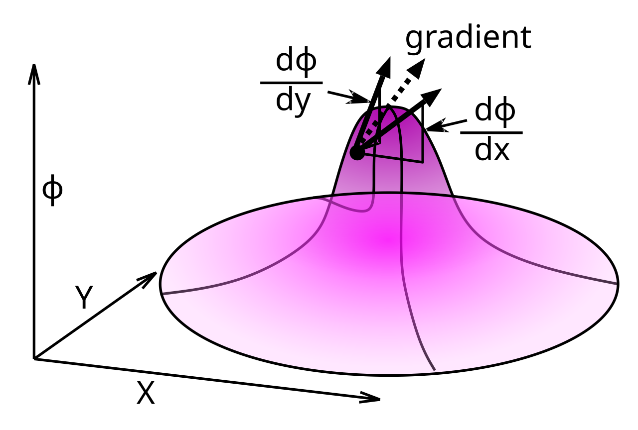
Figure 1: Computation of the spatial gradient using all 18 neighbors that have a non-zero projection along a given axis (in this case, looking at the x axis). The two face points (\(+,-\) along the axis) have a full projection along the axis, and thus enter with a weight of 1. The 8 edge points each have a \(\frac{1}{\sqrt{2}}\) projection of their overall distance along the axis, and thus contribute with that overall weighting. Similarly, the 8 corners have a \(\frac{1}{\sqrt{3}}\) projection weighting. In computing the weighted average, the sum of all neighbor differences is divided by the sum of the weighting terms.
In three dimensions, the computation can be made more accurate and robust by including more of the neighbors, just as we did for the computation of the Laplacian \(\nabla^2\). The most relevant neighbors are the 18 that have some projection along an axis, as illustrated in Figure 1. These can be organized into 9 rays that project through the central point, so that the above approximation can be extended to:
\[ \frac{1}{(2 + \frac{8}{\sqrt{2}} + \frac{8}{\sqrt{3}})} \sum_{j \in N_{9}} k_j (\phi_{j+} - \phi_{j-}) \]
Where the neighborhood \(N_9\) contains pairs of points \(j+\) and \(j-\) that are opposite ends of the 9 rays through the central point, and the distance weighting factors \(k_j\) are:
- • faces: \(k_j = \pm 1 \)
- • edges: \(k_j = \pm \frac{1}{\sqrt{2}} \)
- • corners: \(k_j = \pm \frac{1}{\sqrt{3}} \)