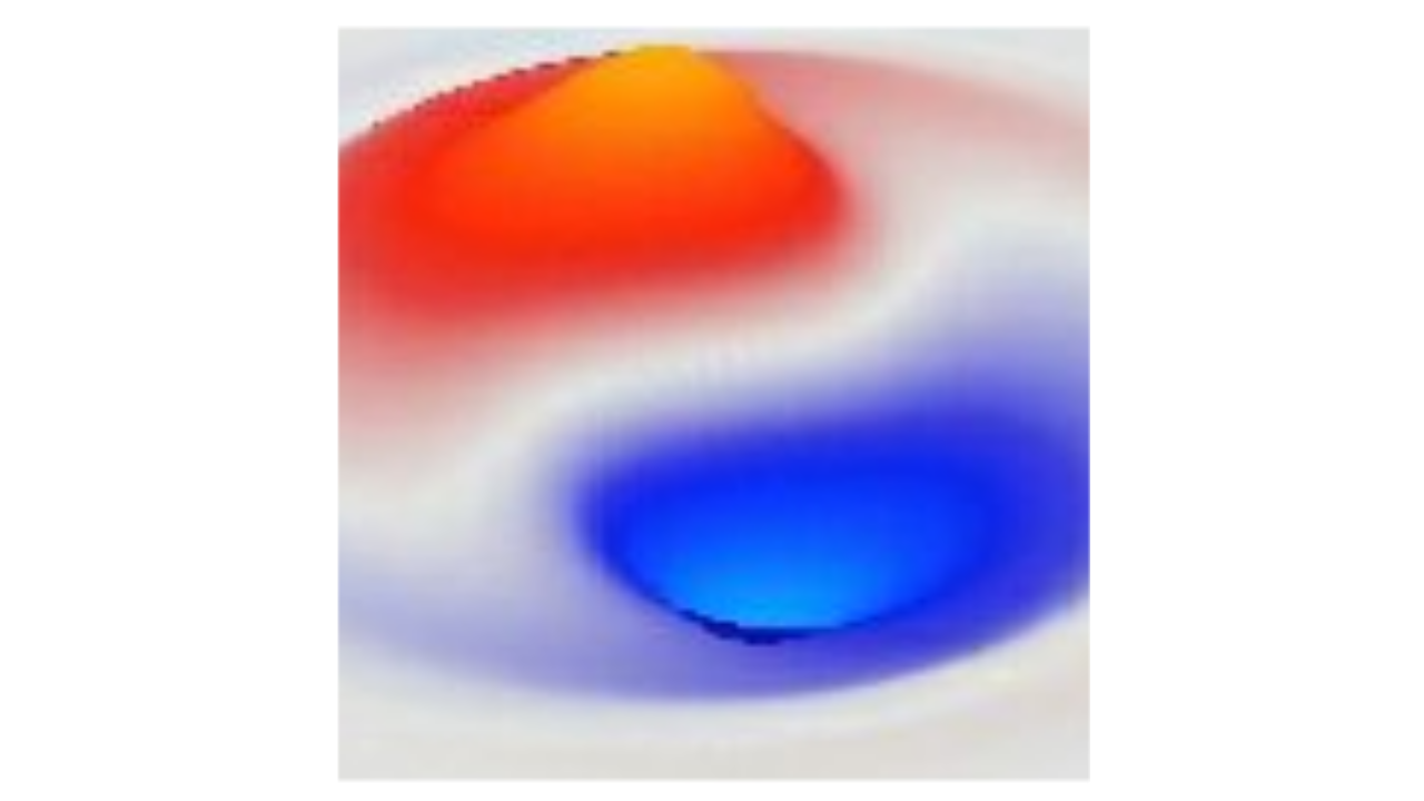
Maxwell Simulation
From units
Config • ViewInterval
Config • Wavelength
Config • PacketWidth
Config • PacketSlab
Config • Amplitude
Config • Source
Config • Polarization
Y
Config • Velocity
Params • Edges
Fixed
Wrap
Damp
Params • C
Params • A0NoWave
Params • Mu0
Params • Eps0
Units
Units
GUI
GUI
Update
Panel:
Plane
ZeroCtr
Current
Counters:
Move:
Rot:
Pan:
Save:
Open CSV
Filter
Unfilter
This simulation runs the Maxwell wave equations. There are multiple sections exploring different electromagnetic (EM) wave phenomena. This should be helpful in better understanding the relationship between the four-potential \(A_\mu\) and the electrical vector field E which is the gradient of the potential, and B which is the curl of it.
Electrical potential
The electrical potential \(A_0\) is represented by the value A0s in the simulation. The default Electric Potential sim_em:Config sets up a fixed point charge at the center of the state space (see the Source in Config entries at the left-hand side for the location: -1 means the center).
As you sim_em:Step 1 this simulation, you can see the A0s value spread out to the \(1/r\) curve that then corresponds to a \(1/r^2\) curve in terms of the gradient of A0s, which is what drives the force on another charged particle.
The Charge Dipole Config is similar, but sets up two opposite charges, where you can see that the distant field state falls off as \(1/r^3\) because the two opposing potentials largely cancel each other out, leaving a small residual.
The A0NoWave flag in Params controls whether the updating of the A0s value uses the diffusion equation (A0NoWave = true) or the standard wave equation (A0NoWave = false). In the diffusion equation, the neighbor-based potential force generated by the Laplacian is applied directly to the velocity, instead of adding to the existing velocity factor, like an acceleration term should. When this is on (as it is by default), it makes the A0 potential propagation more robust, and more similar to the Coulomb gauge.
EM waves
The Linear Polarization config creates an EM wave with linear polarization in the E and B fields along the transverse dimensions. The three other panels show the A, E and B fields using the Vector display, which shows the X,Y,Z components as vector lines pointing in the direction of these vector fields.
Press Step 1 a few times and you’ll see all the vector fields light up. You can use your mouse scroll functionality to zoom into the 3D display to get a better view of the vectors (also the bottom toolbar Zoom in button too). You should see that the A vector potential is pointing up and down in the Y direction, which causes a corresponding E gradient in the same Y axis, while the B field is in the Z axis due to the way that the curl works.
Thus, you can see the expected phenomenon where the E and B waves oscillate 90 degrees out of phase with each other, along the two different transverse axes (Y and Z) relative to the direction of wave travel (X).
The Polarization axis is selectable in the Config settings.
The Circular Polarization config creates a circularly polarized wave configuration, which just has a different phase relationship that emerges in the E and B fields.
Charge current source
The Moving Charge configuration simulates a moving beam of electrical charge current, along the X axis, which allows you to see the resulting magnetic B waves created surrounding this current. Use the Up and Down arrow buttons on the lower view toolbar to move the Y plane slice up and down, to see how the B field curls around the moving charge.