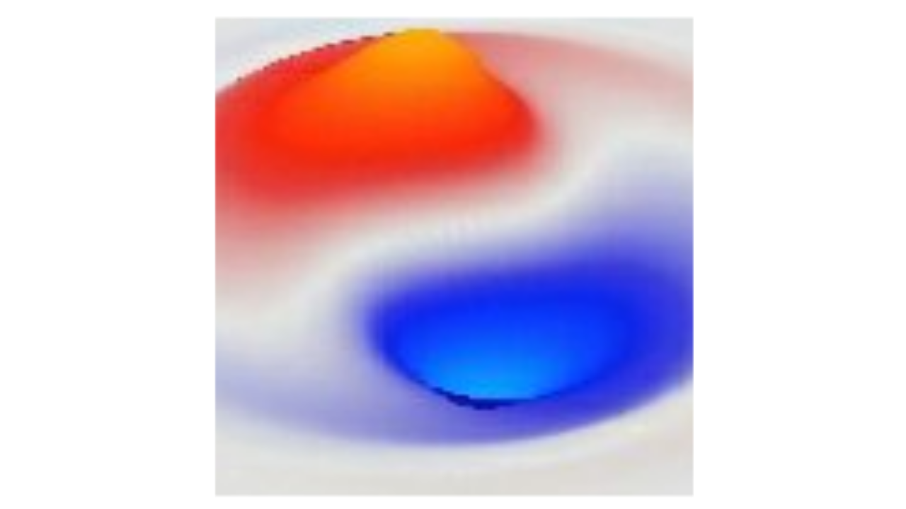
Schrodinger 1D Simulation
From units
Config • ViewInterval
Config • Wavelength
Config • PacketWidth
Config • PacketSlab
Config • Amplitude
Config • HydrogenRadius
Config • OscillatorPeriod
Params • Edges
Fixed
Wrap
Damp
Params • Hbar
Params • Mass
Units
Units
GUI
GUI
Update
Panel:
Bars
ZeroCtr
Current
Counters:
Move:
Rot:
Pan:
Save:
Open CSV
Filter
Unfilter
This simulation runs the Schrodinger equation in 1D. See also Schrodinger 3D Simulation for the 3D version.
In general, the sim_sch1d:Root Stats Plot shows that the overall Mag magnitude of the wave across space remains constant over time: this is the conserved probability value, because the Schrödinger equation has a unitary update property, effectively rotating through the complex plane.
The sim_sch1d:Config options include:
• Free Packet: is like the wave packet option in the KG 1D simulation. The most salient property of this case here is that the waves spread out (disperse) much more quickly than in the KG case. This property is analyzed in complex waves.
• Harmonic Oscillator: is the widely-studied case of the quantum harmonic oscillator, which uses the V potential to trap the wave state within a confined region, where it oscillates back and forth (click on the V variable to see the shape of this well). This case shows that the stable states have integral energy differences, and that the lowest energy state still has a non-zero amount of energy: the complex number system is always rotating, and is therefore never actually sitting still. This is relevant for the zero point energy and associated theories.
• Box Standing Wave: puts a wave state precisely between two fixed walls. If you click on sim_sch1d:Mag you can see that the magnitude of the wave remains constant over time. It is a good idea to set the View Interval config value to 10 or 100 to speed this up.
• Box Two States: are the two lowest standing waves superimposed. They exhibit a complicated beat-frequency oscillation overall.
• Hydrogen Ground: simulates a simple version of the Hydrogen atom, as Bohr did back in the day, showing how the wave is trapped in an S type orbital with a discretized frequency. This looks better in the 3D version.
• Hydrogen P: simulates the excited P orbital state. Likewise looks better in 3D.