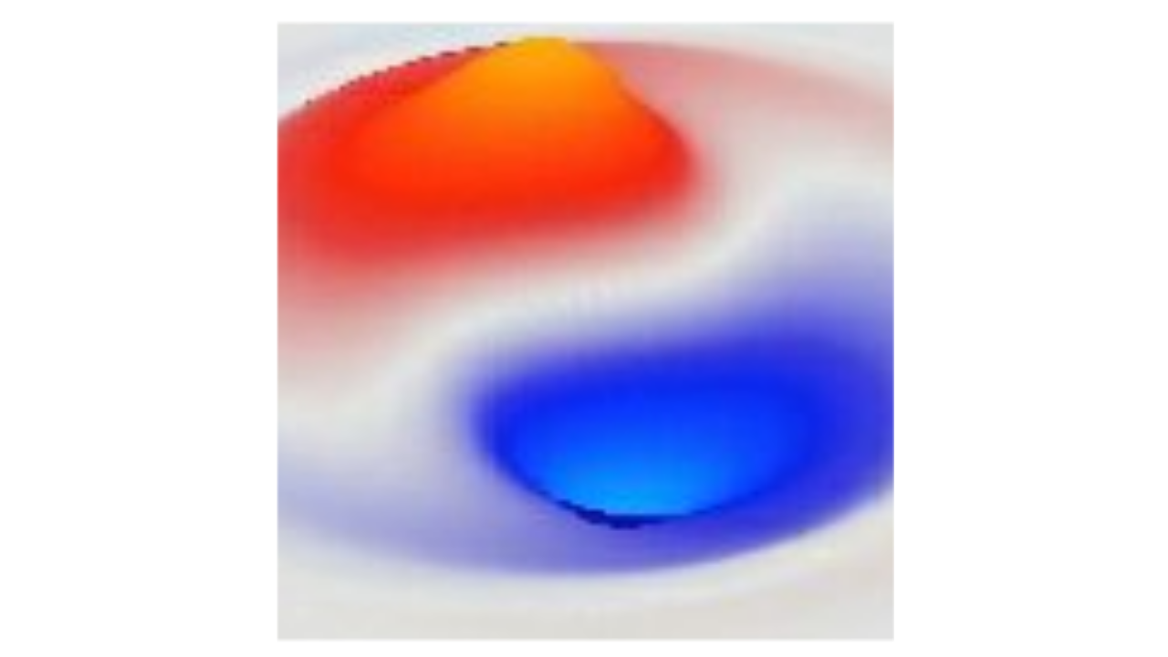
Lagrangian
Lagrangian mechanics was formulated by Joseph-Louis Lagrange, in collaboration with Leonhard Euler, in 1788, providing a powerful way of understanding classical Newtonian physics. It also plays a critical role in the Standard Model, where it is used to define the gauge invariances that define the way that forces interact with particles.
The Lagrangian (not to be confused with the Laplacian that computes the spatial gradient of the wave), is typically defined as the total kinetic energy T minus potential energy V:
\[ \mathcal{L} = T - V \]
By comparison, the Hamiltonian formulation (proposed in 1833) defines the total energy as the sum of kinetic and potential energy:
\[ H = T + V \]
The use of the T symbol to represent kinetic energy captures the fact that this is typically a purely time-dependent factor, reflecting the rate of change in state over time (i.e., velocity) (squared). The potential energy is a complementary space-dependent factor. For example, in the standard wave equation context, the potential energy is a function of the spatial gradient (Laplacian) of the wave state. The same division holds for the harmonic oscillator, where the kinetic energy is in terms of velocity, while the potential energy is in terms of the height (displacement) of the mass-on-a-spring.
Thus, in the context of the four-vector notation that is particularly useful in applications of the Lagrangian, the Lagrangian has a covariant metric tensor (Time minus Space), while the Hamiltonian has a contravariant metric (Time plus Space).
The action
The Lagrangian is used to evaluate the action \(S\), which is a path integral between two points (i.e., two distinct states of the overall system):
\[ S = \int \mathcal{L} dt \]
\[ S = \int_{q_1}^{q_2} \mathcal{L}(\dot{q}, q) dt \]
Where the latter expression provides the concrete parameterization of the two points \(q_1\) and \(q_2\), and the Lagrangian being a function of the individual points along the way between these two points (i.e., the path), and the velocities along these paths.
The q points are coordinates in the configuration space of the system, which are typically strategically chosen to simplify the computation, and in general expand exponentially in the number of dynamic elements in the system.
In general there are infinitely many paths that the system might take between any two states, and the key question that the Lagrangian approach answers is: which path is actually taken?
The answer to this question differs in a particularly compelling way between the classical (Newtonian) and quantum approaches. In the classical approach, there is indeed a single “best” path taken, and it is determined by the principle of least action: The path taken is the one that minimizes the value of the action path integral.
In effect, this principle says that the path taken by a particle described by a Lagrangian will minimize the difference between kinetic and potential energy over time. In other words, it will convert between these two forms of energy in the slowest way possible.
By contrast, in the quantum mechanical approach, all possible paths are taken in parallel, and they each contribute according to the sum of the phases of the paths converging on each end point. In other words, the quantum wave explores all possible paths in parallel, exhibiting the kinds of interference patterns shown in the double slit experiment. This is consistent with the pilot wave duality, where the wave serves as a kind of antenna for the particle. While it is physically implausible for a particle to explore all possible paths in parallel, this is precisely what a wave is good for.
Euler-Lagrange laws of motion
The action effectively defines the Euler-Lagrange equation which can be used to derive laws of motion.
\[ \frac{d}{dt} \left( \frac{\partial \mathcal{L}}{\partial \dot{q}_j} \right) = \frac{\partial \mathcal{L}}{\partial q_j} \]
By substituting the Lagrangian into this equation, the equations of motion for the elements of the system can be derived.
The left-hand-side of this equation is the 2nd order temporal derivative, and the right-hand-side is the spatial gradient, so this is in fact identical to the standard wave equation dynamics. Nevertheless, it can be derived as the solution that makes the action stay at a critical point (e.g., a minimum), providing an independent pathway to arriving at the same place.
Simple harmonic oscillator
The simple harmonic oscillator (SHO) case provides a simple illustration of the Lagrangian, where we can derive Newton’s laws of motion.
The Lagrangian as kinetic – potential energy is:
\[ \mathcal{L}(x,\dot{x}) = \frac{1}{2} m \dot{x}^2 - V(x) \]
where the potential energy function is:
\[ V(x) = \frac{1}{2} k x^2 \]
To apply the Euler-Lagrange equation, we have the following derivatives:
\[ \frac{\partial \mathcal{L}}{\partial x} = - \frac{\partial V}{\partial x} \]
\[ \frac{\partial \mathcal{L}}{\partial \dot{x}} = m \dot{x} \]
\[ \frac{d}{dt} \left( \frac{\partial \mathcal{L}}{\partial \dot{x}} \right) = m \ddot{x} \]
Therefore:
\[ m \ddot{x} = - \frac{\partial V}{\partial x} \]
which results in the Newtonian equations for the SHO using the potential energy function:
\[ m \ddot{x} = -k x \]