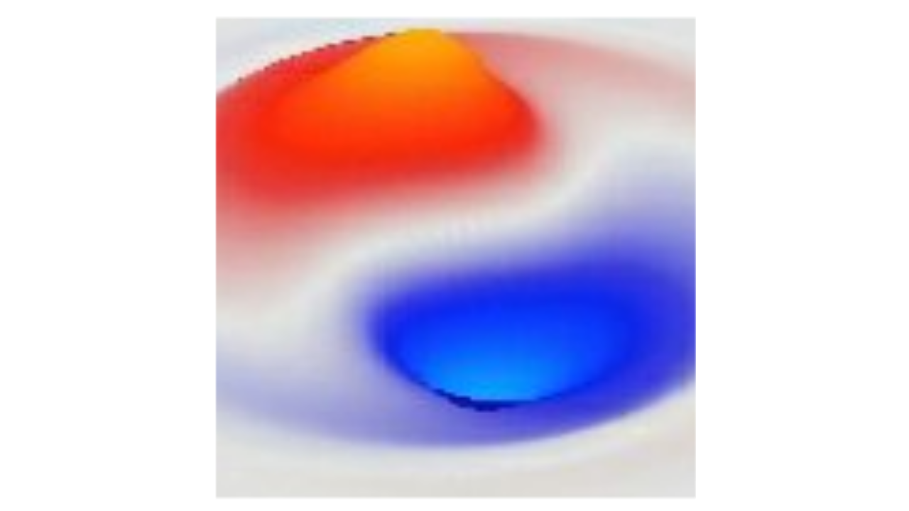
Hamiltonian
Using special relativity, plus the notion of conservation of energy — i.e., that the total energy of the system is strictly conserved over time, we can derive the Klein-Gordon (KG) equation from first principles. In keeping with physicists’ penchant for assigning people’s names to concepts that would otherwise be very easy to understand if just spelled out, the total energy of the system is also called the Hamiltonian (\(H\)), and standard Newtonian physics can all be derived from the appropriate Hamiltonian (which is what W. R. Hamilton did).
The Hamiltonian formulation is a version of Lagrangian mechanics, which predated it, and both formulations play a critical role in the Standard Model.
This motif of using the total energy of the system to derive basic physical laws seems to work quite well in many cases, and is thus the primary way that such laws are derived for different definitions of the total energy. Essentially, the physical laws are latent in any given definition of total energy, and really amount to specifying the dynamics by which energy gets moved around in different ways, without ever gaining or losing any total energy.
This Veritasium video is strongly recommended for the history of the development of this approach, which started with the principle of least action developed originally by Pierre Louis Maupertuis. The second video in this series of two shows how this same principle applies to the path integral formulation of quantum mechanics, and compellingly demonstrates how quantum waves really must be spreading out through space in order to find the right path for a particle to take.
In anthropomorphic terms, the quantum wave function is like a perceptual system for particles, telling them how to move in order to go in the most efficient way! And the Hamiltonian provides a mathematical framework for defining what “the most efficient way” actually means.
The form of the total energy that is used as a starting point determines the scope of the physics that the resulting equations of motion support. The KG equations are derived directly from the relativistic total energy (from Einstein’s special relativity), so they therefore automatically produce all of those relativistic phenomena. However, Schrodinger’s equation is derived from a Newtonian total energy function, which means that it does not handle relativistic phenomena.
The Hamiltonian can be extended to include spin and coupling to the EM field, to derive the Dirac equation (which is just a more complicated version of the KG equation). You will see that the total energy equation and the corresponding wave equation are very directly related mathematically, and thus this overall approach of using the total energy to derive the wave equation is a very powerful tool that is important to understand if you want to really understand what these wave equations are doing.
You should be familiar with our computation of the total energy associated with a simple wave, which we calculated in waves. There we saw that for each cell element in our wave matrix, the total energy was the sum of the kinetic and potential energy, where kinetic energy is a function of how fast the state value is moving, and potential energy is a function of how much stress or tension there was between the state and its neighbors (i.e., the curvature of the space).
Now, we’re going to try to formulate the total energy associated with the “particle” represented by the entire wave function, instead of thinking in terms of each individual cell within the wave state. We’ll see that we can compute the resulting total particle energy using local cell-level calculations, but the motivations and logic are different. There are still kinetic and potential contributions to this overall particle energy, but it is the overall velocity (actually momentum, which is just velocity times mass) of the particle, not the individual cell state, that we are concerned with in computing the kinetic energy.
As discussed in special relativity, the relativistic total energy of a particle moving with momentum \(\vec{p}\) and having a rest mass \(m_0\) is given by the following equation:
\[ E^2 = \vec{p}^2 c^2 + (m_0 c^2)^2 \]
\[ E = \sqrt{\vec{p}^2 c^2 + (m_0 c^2)^2} \]
The fact that these two components of energy, momentum and rest mass, add together only when squared, ended up causing a remarkable amount of grief and confusion about the meaning of the KG and Dirac equations. Taking the square root of a sum is not a very friendly mathematical operation, and it automatically leads to the possibility of both positive and negative valued solutions. We are able to largely avoid these problems in our overall approach, however, in part by just using the squared energy instead of the raw energy. If the energy is conserved, so is its square!
To do anything with this total energy equation, we need to be able to compute the momentum and the energy values from our wave states. We have already indicated that the momentum (velocity) of the wave is proportional to the amount of curvature in the wave state — more curve = faster velocity. This can be formalized with the appropriate constants in the following momentum operator (the little hat \(\hat{}\) indicates that this is an operator to be applied to a wave state) which operates over each cell in the entire wave state to produce the associated momentum of the particle:
\[ \hat{p} = -i \hbar \vec{\nabla} \]
We highlight this because we’ll keep using it again and again as we work our way up to the Dirac equation. Do not be alarmed by the presence of the \(-i\) imaginary number at the start of this equation — we’ll get rid of it soon enough. See complex numbers for more information if you want to brush up on your knowledge of these seemingly strange numbers at this point — you’ll need to really understand them in detail to understand the Schrodinger equation. They really are very simple once you get past all the imaginary business and recognize their actual practical application.
The total energy operator for the wave state is computed in terms of the overall rate of change across all the wave cells, consistent with the notion that energy is a function of the velocity (kinetic energy) of the cell states:
\[ \hat{E} = i \hbar \frac{\partial }{\partial t} \]
again we see the imaginary number and \(\hbar\) constants here.
To see how this all fits together, we now substitute in these operators in place of the momentum and energy terms in the above energy equation (squared version), and have them operate on the wave state values. The imaginary numbers turn into 1’s and -1’s in the process of the squaring, and thus very kindly disappear:
\[ E^2 = \vec{p}^2 c^2 + (m_0 c^2)^2 \]
\[ -\hbar^2 \frac{\partial^2 {\phi}}{\partial t^2} = \left (-\hbar^2 \nabla^2 c^2 + (m_0 c^2)^2 \right) \phi \]
\[ \frac{\partial^2 {\phi}}{\partial t^2} = \left( c^2 \nabla^2 - \frac{(m_0 c^2)^2}{\hbar^2} \right) \phi \]
\[ \frac{\partial^2 {\phi}}{\partial t^2} = c^2 \left(\nabla^2 - \frac{m_0^2 c^2}{\hbar^2}\right) \phi \]
And amazingly, at the end, we recover exactly the Klein-Gordon equation!
This means that the propagation of the particle defined by a KG wave function will conserve the total relativistic energy over time, simply by virtue of following the local wave dynamics. This means that a KG wave-particle will obey the physics of special relativity in every way. And in the case when the wave velocity is low compared to the speed of light, then the system will behave according to the laws of Newtonian physics, because special relativity reduces to standard Newtonian physics in this case.
In short, Eq 4 contains such a huge scope of physics in such a simple package — it is truly the most efficient representation of the essence of physics. Nevertheless, it is not sufficient to describe any actual physical particle, except perhaps the Higgs boson.
Four-Vector Version
Before continuing, we explore the ultra-compact version of the above derivations that is possible using the four-vector space-time coordinate system introduced in maxwell. In this system, the four-momentum operator is defined as:
\[ {\hat{p}^\mu} = i \hbar \partial^\mu \]
\[ = i \hbar \left(\frac{\partial {}}{\partial {ct}},-\frac{\partial {}}{\partial {x}},-\frac{\partial {}}{\partial {y}},- \frac{\partial {}}{\partial {z}}\right) \]
\[ = i \hbar \left(\frac{\partial {}}{\partial {ct}}, -\vec{\nabla} \right) \]
\[ = \left(\frac{\hat{E}}{c}, \hat{p}\right) \]
As indicated, it should be clear that the first (time) component of this is the energy operator given above, while the spatial components are the momentum operator (Eq 2):
\[ \hat{E} = i \hbar \frac{\partial}{\partial t} \]
\[ \hat{p} = -i \hbar \vec{\nabla} \]
If you then square this momentum operator (using the standard covariant, contravariant four-vector definition of multiplying vectors), you get:
\[ {\hat{p}^\mu} {\hat{p}_\mu} = \frac{\hat{E}^2}{c^2} - \hat{p}^2 \]
Now this is quite interesting, because it can be directly related to the relativistic energy-momentum equation:
\[ E^2 = \vec{p}^2 c^2 + (m_0 c^2)^2 \]
\[ \frac{E^2}{c^2} = \vec{p}^2 + m_0^2 c^2 \]
\[ \frac{E^2}{c^2} - \vec{p}^2 = m_0^2 c^2 \]
So we can now put these two equations together, to get:
\[ {\hat{p}^\mu} {\hat{p}_\mu} = m_0^2 c^2 \]
Now, we also know that the wave equation arises from the second-order derivatives of a four-vector:
\[ \partial_\mu \partial^\mu = \frac{1}{c^2}\frac{\partial^2 {}}{\partial t^2} - \nabla^2 \]
and this four-momentum operator is essentially just a first-order derivative with some additional constants (including the \(i\) term, which, when squared produces a \(-1\)), so when we apply these operators to our wave variable \(\phi\), we get:
\[ {\hat{p}^\mu} {\hat{p}_\mu} \phi = m_0^2 c^2 \phi \]
\[ i^2 \hbar^2 \partial_\mu \partial^\mu \phi = m_0^2 c^2 \phi \]
\[ - \hbar^2 \left(\frac{1}{c^2}\frac{\partial^2}{\partial t^2} - \nabla^2\right) \phi = m_0^2 c^2 \phi \]
\[ \frac{\partial^2 {\phi}}{\partial t^2} = c^2 \left(\nabla^2 - \frac{m_0^2c^2}{\hbar^2}\right) \phi \]
Which is right back to our KG wave equation.
In summary, the core of the KG wave equation, and of special relativity, and much of quantum mechanics, can all be reduced to this one simple equation:
\[ \hat{p}^\mu \hat{p}_\mu \phi = m_0^2 c^2 \phi \]
This is in some sense the most fundamental equation of the universe, subsuming the more popular \(E = m c^2\) and, as we’ll see, providing the basis for further extensions to the KG equation.